Here is the tiny clever bit from last night’s demodulation experiment using HF radiofax. For the purposes of this experiment, I record a single channel audio of the HF fax transmission. The audio is centered at an audio frequency of 1.9 Khz, and varies (except for start/stop pulses) between 1500 and 2300 Hz. I begin by band pass filtering using a filter designed with the applets you can find at this website, then split the signal into two halfs, and multiply one half by a sine at 1900 Hz, the other by a cosine at 1900Hz. This works just like a I/Q mixer in a software defined radio (in fact, it is just such a mixer). This frequency shifts the signal down so that now all signals occur between -400 and +400 hz.

From each pair of I, Q values, we can easily determine the squared amplitude of the signal (just I² + Q²) or the instantaneous phase of the signal (atan(I/Q)) but we are interested in the frequency: the _change_ in phase between two samples. I’ve sen this derived before, but this way makes the most sense to me, so I thought I’d write it down.

Let’s consider two adjacent I/Q samples, I₀ Q₀ and I₁ Q₁. The question is, what is the angle that will rotate sample zero to sample one? Well, first, we must realize that they may differ in amplitude. We’re not concerned about their amplitude, so we might as well get to normalizing them. We simply divide them through by their length. That’s no problem. But then how do we compute the angle between them?

I chose to use the geometric interpretation of cross products to figure out the math. If we have two three-dimensional vectors, and compute their cross product, the resulting vector is perpendicular to both, and has length proportional to product of the length of the two vectors and the sine of the angle between them. In our case, our vectors seem like two-dimensional vectors, but let’s fix that simply: tack on an extra zero to each pair. They are now obviously both contained in the X-Y plane, we know that the normal is perpendicular to that plane so has zero components for both the X-Y entries, and the Z component contains all the interesting bits. In particular, we know that its proportional to the length of the two vectors (which are both one, since we normalized, and can be ignored) and the sine of the angle between them. Hence, we could just take the arcsine, and recover the angular change (which would be between -π/2 and &pi/2). We can then map this back into frequencies if needed (-samplerate/2 to +samplerate/2) or in our case, map that into grayscale values.

But surely you are balking at this ugly arcsine call in the middle of our program, aren’t you? Well, it’s not like we haven’t got CPU to burn. The implementation I have processes 15 minutes of recorded audio in just a few seconds, so even using an arcsine results in a program which is 100 times faster than realtime on current hardware. But you are right: it worried me a bit, so I scratched a little deeper. When you have sines and cosines in things, it’s often useful to use small angle approximations. These are derived from the Taylor series expansions for sine and cosine.

For small x (values near zero) cosine(x) is approximately one, and sine(x) is approximately x (just take the first term of each of the above equations. But, if sin(x) is just about x, that means that the asin(x) is just about x too. Thus, we can choose to not use asine at all, and instead just use the output of our cross product calculation as our frequency, and we might expect it to work just fine (it has range -1 to 1, whereas asin has range -π/2 to π/2, but the frequencies we are interested in are confined to a small portion of the audio spectrum anyway, so the error is likely to be minimal).

If you want, you could try to use more terms from the series for arcsine:

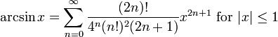
but in my experimentation, it made no difference in image quality.

Anyway, once you recover frequency, you want to map values from near -400 hz to black, and 400 to white. You need to normalize for sample rate, some clamping, and some resizing, and you are done. Okay, I haven’t covered rectification/slope correction, and the aspect ratio stuff is a bit tricky to get exactly right, but I’m still working on them.

Hope this wasn’t too boring.