Rob (AK6L) was interested in my recent experiments in slow scan television, but didn’t know much about color spaces. It’s an interesting topic on many fronts, and I thought I’d write a brief post about it here to explain it to those who may not be familiar.
Consider this nice 320×240 test image of Wall-E that I’ve been using:
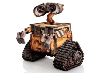
Most of you probably know that these images are really combinations of images in three different colors: red, green and blue. If you take a magnifying glass and look at your TV, you’ll see that your television displays images as a combination of glowing red, green and blue dots. If we instead split this color image into separate images, one for red, one for green, and one for blue, and display each one separately, we can see the image in a different way:
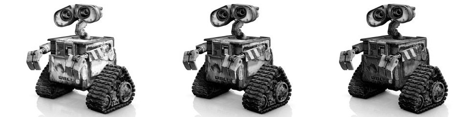
One thing to note: there is lots of detail in each of the three sub-images. That means that there is considerable redundancy. When data streams have lots of redundancy, that means there is an opportunity for compression. Compression means we can send data more quickly and more efficiently.
So, how can we do this? We transform the RGB images we have into a different set of three images, where most of the visual information is concentrated in one channel. That means we can spend most of our time sending the dominant channel, and less effort sending the other channels, maybe even sending lower resolution versions of those channels.
But how do we do that? Well, let’s do some magic, for each pixel in the image, let’s compute a new image Y from the R, G, and B images. Y will consist of 30% of R, 59% of G and 11% of B. This computes a representative black and white image from the R, G, and B channels. (If you didn’t know a lot about color science, you might just try averaging R, G, and B, but your eyes have different sensitivity to R, G, and B light. If you use the proportions I describe, you’ll get a lot better subjective match to the value of each pixel.) Then, let’s compute two additional channels, the channel that consists of R – Y, and the channel that consists of B – Y.
If you are mathematically inclined, you’ll see that this process is invertable: no information is actually lost. Given the Y, R-Y and B-Y images, we can recover the RGB images. But what do these images look like?
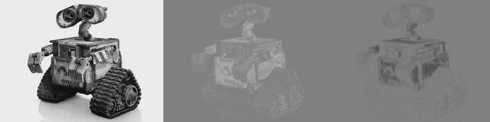
(Since R-Y and B-Y may be negative, we actually compute (R-Y)/2 + 0.5 and similar for B-Y).
Neat! Now, the most detail is confined into the Y image. In the Robot 36 SSTV mode, each scanline spends 88ms transmitting the 320 pixels for the Y channel. The R-Y and B-Y channel are first downsampled (resized down) to just 160×120 (half size in both dimensions). Robot 36 takes just 44ms to send each of those. But because we’ve resized down in Y, we only have half as many scanlines in R-Y and B-Y channels. So Robot 36 operates by sending one 320 pixel row for Y, then one 160 pixel row for R-Y, then the next 320 pixel row for Y, then one 160 pixel row for B-Y. Each pixel in the R-Y and B-Y channels will then cover 4 output pixels.
I’ve glossed over a lot of details, but that’s basically how color spaces work: we convert an image into an equivalent representation, and then transmit some channels at lower resolution or lower fidelity than the others. This idea also underlies image compression technology like JPEG.
Addendum: I generated the images above using gimp. If you go to the Colors…Decompose menu, you can bust images into three different RGB images, or YCrCb.