Category Archives: Math

How is PWM modulation like AM modulation?

In thinking about the 555 timer AM transmitter that I constructed last night and trying to understand how it might work, I eventually ended up with a basic question about PWM modulation. It boiled down to this: if you are generating a pulse width modulation signal with a rate of (say 540khz) but pulses whose duty cycle varies from 0 to 100%, how does this implement AM modulation?

If we consider the rectangular pulse centered inside an interval of running from -1 to 1, then a pulse with a duty cycle of D percent runs from -D/100 to +D/100. (From now on, we’ll find it convenient to express D as a fraction and not as a percent). We can use Fourier analysis to decompose this square wave into a series of sines and cosines at multiples of the base rate. For our application, we can ignore the DC component (it’ll be trimmed off by a DC blocking cap anyway) and we can assume that all higher multiples of the carrier frequency will be low pass filtered. The only thing we really need to look at is the component right at the carrier frequency.

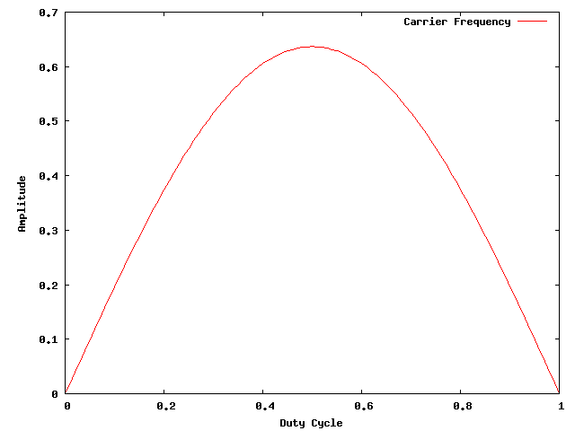
We can do this analytically without too much trouble. To compute the Fourier coefficient, we compute 1/L * integral(cos(n * pi * t / L), dt, -D, D). (Sorry, WordPress isn’t all that good at this, and I wasn’t able to get MathJax to work). If we think of the the complete cycle as going from -1 to 1, then L = 1, and we can work this out: the amplitude of the carrier turns out to be 2.0 * sin(π * D) / π. We can make a graph, showing what the amplitude of the sine wave at the carrier frequency will be for varying duty cycles.

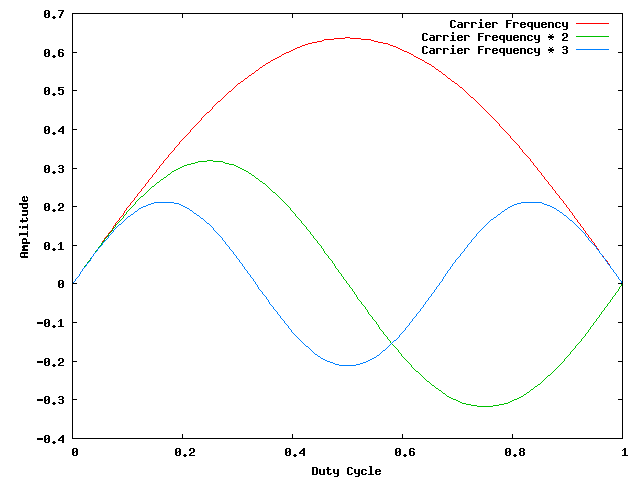
What does this mean? If we shift the duty cycle of our PWM waveform, we actually are modifying the amplitude (and therefore the power) of the transmitter output at the carrier frequency. As we deviate more from 0.5, we get more and more energy in the higher harmonics of the carrier frequency.

I’m sure that was about as opaque an explanation as possible, but it suggests to me a simple software simulation that I might code up this weekend to test my understanding.

Stay tuned.

Addendum: We can work out the relative amplitudes of the first three multiples of the carrier frequency:
HOPALONG, from Dewdney’s Armchair Universe

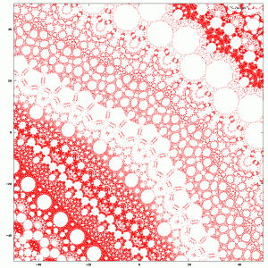
All this fiddling around with the Lorenz attractor has made me try to think of other simple, easy graphics hacks that I could make. I recalled that A.K. Dewdney had some simple graphics hacks in one of his Computer Recreations column back in the 1980s. It turns out that Wallpaper for the mind was published back the September 1986 issue of Scientific American, and was reprinted in Dewdney’s compendium The Armchair Universe. I had a quick look, and wrote the following implementation of the HOPALONG program first… discovered? written? by Barry Martin. The program initializes X and Y to zero, and then repeatedly applies a pair of functions to the existing X, Y to generate new values. The program here just prints the values.

[sourcecode lang=”C”]
#include <stdio.h>
#include <stdlib.h>
#include <math.h>

#define LIMIT 21000000

double sgn(double x)
{
if (x == 0.) return x ;
if (x < 0.0) return -1. ;
return 1.0 ;
}

main(int argc, char *argv[])
{
double x, y ;
// double a = -200, b = .1, c = -80 ;
// double a = 0.4, b = 1, c = 0 ;
// double a = -3.14, b = 0.3, c = 0.3 ;
double a = -1000., b = 0.1, c = -10 ;
double nx, ny ;
int i ;

x = y = 0.0 ;

for (i=0; i<LIMIT; i++) {
printf("%lf %lf\n", x, y) ;
nx = y – sgn(x) * sqrt(fabs(b*x-c)) ;
ny = a – x ;
x = nx ;
y = ny ;
}
}
[/sourcecode]

Depending on the value of a, b, and c, a different set of points is produced. I’ve left several “interesting” values as comments in the code. The set that remains uncommented is actually among the more interesting. It generates all sorts of interesting details. To visualize these points, I found it convenient to use gnuplot. Zooming into a fairly small region, you can see this wonderfully vascular like pattern evolve:

I remember implementing this on my old Atari 400 back then. But I probably didn’t really appreciate how it worked. Now, I recognize that this iteration is some kind of iterated function system, and that you might reasonably expect it to develop these kind of fractal patterns. It seems likely for convergence that the variable b should have absolute value less than 1, but a and c can (I think) be more or less chosen at any scale you desire. The sqrt implements some nonlinearity, which accounts for the many curved features that are visible.

This program has all sorts of fun tweaks. It always begins by initializing x and y to zero, but if you try different starting points, you get different orbits. You could try coloring the dots by slowly changing the way they are colored, or by coloring all points on the same orbit the same color. I removed the sqrt, and still got some interesting patterns. I’ve also thought of producing some animations by slowly varing some of the parameters to see how the resulting pattern evolves. All sorts of good stuff.

The Chaotic Lorenz Water Wheel

Doing a bit more reading, I found out that the equations that make up the Lorenz attractor (which are derived from a simplified model of 2D fluid flow with a superimposed temperature gradient) can also be thought of as governing another physical system. Imagine a water wheel, with a number of buckets spaced evenly around the perimeter. These buckets filled at the top of the wheel. As that bucket fills, any offset will generate an imbalance, and the wheel rotates. That will rotate another bucket into position. The amount of water in that bucket is less because it spends less time under the faucet. But eventually, the buckets all fill up, the wheel is balanced, and the friction of rotation causes the motion to cease.

But now, imagine that each bucket is leaky: that some of its water drains out. What happens then? Well, it turns out that depending on the speed at which the water is pumped in and leaks out, the wheel can exhibit chaotic motion: spinning at radically different speeds and often reversing itself. Very neat. Here’s a video of one with a particularly simple design (you can google for more examples):


This would be a fun garden project.

The Strange Attraction of Strange Attractors…

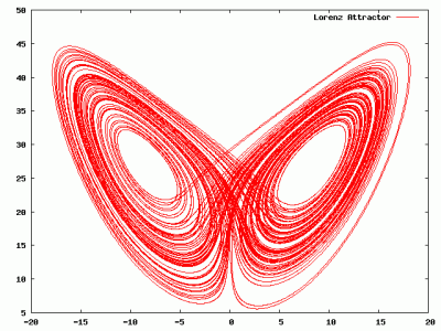
I’ll just lead off with a picture:

This is a graph of the so-called “Lorenz attractor”, first described by mathematician Edward Lorenz in his paper Deterministic Nonperiodic Flow back in 1962. I learned about this kind of stuff probably back in highschool by reading Scientific American. Anyway, the equations themselves are pretty simple, but describe paths which are nonperiodic, and which are unstable: for two points very near each other, their evolution rapidly diverges, and they no longer follow identical paths.

Making these graphs was really just a diversion: I’ve got it in my head that creating an analog circuit that simulates these equations might be a fun thing to do. This is boldly going where others have gone before, so here are some links:

Build a Lorenz Attractor has a nifty little circuit that has two analog multipliers and three op amps. Checking with digikey, the MPY634 multipliers seem pretty spendy for something that is just a lark ($28 a piece, ouch), but Analog Devices makes some devices which seem like they will perform adequately, and cost $8 a piece.

A Simple Circuit Implementation of a Chaotic Lorenz System by Ned Corron uses these less expensive parts (AN633 multipliers, and the super cheapie TL082 op amps) and probably would be a good place to start.

And, of course, we need a YouTube video. Jeri and Chris show off a hardware implementation of the first circuit that Chris assembled:

I didn’t realize until later that the first article was written by Paul Horowitz, one of the authors of the incredible book The Art of Electronics by Horowitz and Hill. Digging a bit more, I found an actual lecture by Paul Horowitz on the subject, posted by user harvardphysics on YouTube:

Addendum: Here are some more links.

From the analogmuseum.org website, a nifty page that points out that if you change the value of the integrating caps, you can effectively change the speed of calculation, allowing the analog computer to directly drive a pen plotter.

I got pointed to the Analog Museum from this page, which in addition to demonstrating the Lorenz attractor running on an analog computer also has schematics and parts lists for actually building an analog computer, again using the AN633 analog multipliers from Analog Devices. Neat.

Happy π day!

It’s 3/14 again, and that means that it’s π day! Huzzah. This year, I thought I’d try implementing a way of computing π which was entirely new to me: finding π hiding inside the Mandelbrot set.

David Boll made a posting back in 1991 to sci.math:

I posted this to alt.fractals about a month ago, and it occurred to me 
  that readers of this newsgroup would probably be interested also. 
  I was trying to show that the 'neck' of the mandelbrot set at (-.75,0) is 
  actually of zero thickness. Accordingly, I wrote a quickie program and 
  started checking the number of iterations that points of the form 
  (-.75,dy) went thru before blowing up (with dy being a small number). 
  Here's a table of results: 
            dy    # of iterations 
            .1             33 
            .01           315 
            .001         3143 
            .0001       31417 
            .00001     314160 
  Notice anything peculiar about the # of iterations? How about the product 
  of the # of iterations with dy? 

Pretty neat. Surf over to his page on the subject for more information and for Gerald Edgar’s proof. I wrote my own implementation which you can find below.
[sourcecode lang=”C”]
#include <stdio.h>
#include <stdlib.h>
#include <stdint.h>
#include <inttypes.h>
#include <complex.h>

/*
* _______
* ( _ ) _
* | | | | _ __ ___ __ _ _ __ __| |
* | | | | | ‘_ ` _ \ / _` | ‘_ \ / _` |
* | | | | | | | | | | (_| | | | | (_| |
* |_| |_| |_| |_| |_|\__,_|_| |_|\__,_|
*
* A program that computes approximations to pi by iterating over
* the Mandelbrot set. Not terrifically useful really, there are
* much faster ways, but this was a way which I had not seen
* before, so I thought it was worth archiving in programmatic form.
*
* Written for pi-day, 3/14/2011 by Mark VandeWettering.
*
* References:
* https://home.comcast.net/~davejanelle/mandel.html
*/

uint64_t
mand(double complex c, uint64_t limit)
{
uint64_t i ;
double complex z ;

z = 0 ;
for (i=1; i<limit; i++) {
z = z*z + c ;
if (cabs(z) > 2.0) break ;
}
return i ;
}

main(int argc, char *argv[])
{
int i ;
uint64_t limit = 10LL ;
uint64_t iter ;
double complex c ;
double y = 1. ;

if (argc == 1) {
printf("computing some approximations to pi using the mandelbrot set.\n") ;
printf(" (close approximations might take a few seconds, warning…)\n") ;
for (i=0; i<9; i++) {
c = -0.75 + y * I ;
iter = mand(c, limit) ;
printf("%9" PRIu64 " iterations, pi is %.8lf, +/- %.8lf\n", iter, 10.*iter/limit, y) ;
y /= 10 ;
limit *= 10LL ;
}
}
exit(0) ;
}
[/sourcecode]

Bonus points: This program when run produces a result which isn’t correct during the last iteration (the Mandelbrot iteration runs to limit, instead of stopping where it should). I suspect that it’s got a bug in it somewhere, and isn’t using enough precision. I’ve just got back from a 24 hour trip to London, a visit from a locksmith (don’t ask) and now 12 hours of sleep, but my brain isn’t functioning right now. Can anyone else spot the issue?

Apollonian Gasket

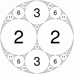
It took me an embarrassingly long time to write a program to generate this fractal known as the Apollonian Gasket:

More information here:

Apollonian gasket – Wikipedia, the free encyclopedia

Each circle is labelled with its curvature (which is simple the reciprocal of the radius). In this particular instance, all the curvatures turn out to be integers. Not really sure why I think this is interesting, but there you are.

Mark’s Bookshelf: Digital Dice by Paul Nahin

Many people use computers to exchange email or pictures, to shop, or even to program for a living. I do all that kind of stuff, but one of the most pleasurable things I do with computers is to use them to answer questions or to gain insight into problems which are too difficult for pen-and-paper analysis.

Digital Dice is a book of probability problems which can be attacked via computer simulation. For the flavor of the sort of problems contained within, consider The Appeals Court Paradox presented in Chapter 16. Quickly, imagine five judges (A, B, C, D, E) who must arrive at a majority decision to overturn a conviction or let it stand. Each justice votes independently, with a probability of yielding the correct decision. For instance, let’s say that A gives the correct decision 95% of the time, with the remaining justices voting correctly 95%, 90%, 90%, and 80%. What is the likelihood that the panel returns the correct decision?

Now, imagine that justice E (who seems to get things wrong much more often than his colleagues) decides to just be lazy and vote along with A (after all, he’s pretty smart, he gets the answer write 95% of the time). What is the probability that the panel returns the correct decision now?

Such problems are fairly hard tedious to work through analytically, but are quite easy to code up as simulations. By tossing dice, and running millions of trials, we can quickly gain insight into a wide variety of problems.

I find this book to be clearly written, and anyone with even a modest amount of programming and mathematical knowledge should be able to complete the projects detailed within. Nahin’s books have been (in my opinion unfairly) criticized by some on Amazon for having the odd typo. I think if that your criticism, you are missing the forest for the trees: the book isn’t meant to be full of code that you type in, it’s meant to challenge you to write your own implementations and experiment. I’ve got several other books by Nahin, and I generally find his style and choice of subject matter to be interesting.

If this is the kind of thing that floats your boat, check it out. Recommended.

Somewhere… over the (simulated) rainbow revisited…

A couple of months ago, I did some simple simulations of light refracting through raindrops in a hope to understand the details of precisely how rainbows form. The graphs I produced were kind of boring, but they did illustrate a few interesting features of rainbows: namely, the double rainbow, and the formation of Alexander’s band, the region of relatively dark sky between the two arcs.

But the pictures were kind of boring.

So, today I finally got the simulation working, did a trivial monte carlo simulation tossing fifty million rays or so, and then generated a picture by converting the spectral colors to sRGB. Et voila!

Horribly inefficient really, but satisfying result.

Addendum: In comparing the results to actual photographs of double rainbows, it seems like my pictures are scaled somewhat strangely (the distance between the arcs seems large compared to the radius). I suspect this is mostly due to the linear projection that I used and the very wide field (the field of view of the camera is nearly 100 degrees, which compresses the center and expands the outside. I’ll have to make some narrower field pictures tomorrow when my mind can handle the math, I’ve reached my limit tonight.

A 2010 “Graphical Computing” Calendar

The Make blog brought the Dead Reckonings blog to my attention. The blog is fascinating: consisting of essays of bits of lost mathematical lore, and nomography in particular. Author Ron Doerfler has some great stuff, and a cool give away: a calendar that demonstrates and explains many different kinds of nomographs. Of course, it’s kind of bad that I discovered the 2010 calendar in October of 2010, but such is life.

Dead Reckonings » A 2010 “Graphical Computing” Calendar.

Drawing “circles” ala Marvin Minsky…

In my re-reading of Levy’s book Hackers, I was reminded of an interesting bit of programming lore regarding an early display hack that Marvin Minsky did for circle drawing. It’s an interesting hack because the lore was that it was originally coded by mistake, and yet the result proved to be both interesting and even useful. I first learned of this years ago when Blinn did an article on different ways to draw a circle, but also learned that it was part of the MIT AI memo called “HAKMEM”. Here’s the basic idea:

One way that you can draw a circle is to take some point x, y on the circle, and then generate new points by rotating them around the center (let’s say that’s the origin for ease) and connecting them with lines. If you have a basic understanding of matrix math, it looks like this:

/ x' \   /  cos theta  sin theta \ / x \
|    | = |                       | |   |
\ y' /   \ - sin theta cos theta / \ y /

(I should learn how to use MathML, but you hopefully get the idea). The matrix with the cosine and sine terms in it is a rotation matrix which rotates a point around by the angle theta. Apparently Minsky tried to simplify this by noting that cos(theta) is very nearly one for small theta, and that sin(theta) can be approximated by theta (we can get this by truncating the Taylor series for both). Therefore, he thought that (I’m guessing here, but it seems logical) that we could simplify this as:

/ x' \   /   1  eps \ / x \
|    | = |          | |   |
\ y' /   \ -eps  1  / \ y /

Okay, it’s pretty obvious that this seems like a bad idea. For one thing, the “rotation” matrix isn’t a pure rotation. It’s determinant is 1 – eps^2 1 + eps^2, which means that points which are mapped move slowly toward away from the origin. Nevertheless, Minsky apparently thought that it might be interesting, so he went ahead an implemented the program. I’ll express it here is pseudo-code:

newx = oldx - eps * oldy
newy = oldy + eps * newx

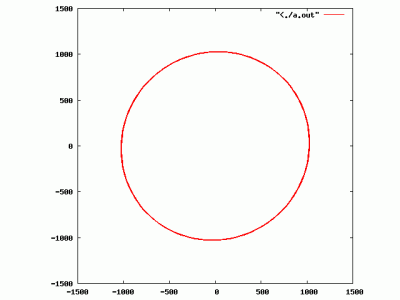
Note: this program is “buggy”. The second line should (for some definition of should) read “oldy + eps * oldx“, but Minsky got it wrong. Interestingly though, this “bug” has an interesting side effect: it draws circles! If eps is a power of 2, you can even implement the entire thing in integer arithmetic, and you don’t need square roots or floating point or anything. Here’s an example of it drawing a circle of radius 1024:

Well, there is a catch: it doesn’t really draw circles. It draws ellipses. But it’s still a very interesting bit of code. The first thing to note is that if you actually write down the transformation matrix that the “wrong” equations implement, the determinant is one. That helps explain why the point doesn’t spiral in. But there is another odd thing: if you implement this in integer based arithmetic, it’s eventually periodic (it doesn’t go out of control, all the round off errors eventually cancel out, and you return to the same point again and again and again). In HAKMEM, Schroeppel proclaims that the reason for the algorithm’s stability was unclear. He notes that there are a finite number of distinct radii, which indicates that perhaps the iterative process will always eventually fill in the “band” of valid radii, but the details of that seem unclear to me as well. I’ll have to ponder it some more.

Addendum: The real reason I was looking at this was because the chapter in Hackers which talks about Spacewar! also talks about the Minskytron whose official name was TRI-POS. It apparently uses some of this idea to draw curves in an interesting way. HAKMEM item #153 also suggests an interesting display hack:

ITEM 153 (Minsky):
To portray a 3-dimensional solid on a 2-dimensional display, we can use a single circle algorithm to compute orbits for the corners to follow. The (positive or negative) radius of each orbit is determined by the distance (forward or backward) from some origin to that corner. The solid will appear to wobble rigidly about the origin, instead of simply rotating.

Might be interesting to implement.

Addendum2: I goofed up the determinant above, it should be 1 + eps^2, not 1-eps^2. Corrected.

Martin Gardner, 1914 – 2010

Today, someone who had a big influence on my life (and whom I’ve never met) passed away: legendary recreational mathematician Martin Gardner. I learned about it from Phil Plait, of the Bad Astronomy blog, courtesy of his twitter feed. Phil writes up his own thoughts here:

Martin Gardner, 1914 – 2010 | Bad Astronomy | Discover Magazine.

I was first exposed to Gardner’s writings in Mathematical Games when I was still in grade school. Our local library used to give away books that they no longer wished in their collection, and at one point, they discarded a couple of decades worth of Scientific American. As a voracious reader of science, I carted dozens of issues home in my book bags over the span of a few days. While I had a wide variety of interests, I read two columns out of nearly every issue: C. L. Stong’s Amateur Scientist and Gardner’s Mathematical Games.

Others will cite Gardner’s greatest contributions as a skeptic, but the lasting impact that he has on me is conveying the mystery, the magic, and the fun of mathematics. It was through his pages that I first learned of John Conway’s “Game of Life” and cellular automata. Of the game Hex. Of Penrose tilings. Of public key cryptography. Of polyominoes. Of game theory. Flexagons. Polygonal dissections. Of machine learning. And dozens of puzzles that intrigued me for hundreds of hours.

I have eight or nine of his books, and still enjoy perusing them for puzzles I haven’t attacked before. His columns were often on cutting edge bits of mathematics, but neither tried to pander to the lowest common denominator, nor to be accessible to only a small mathematical priesthood: his work was accessible and challenging. He basically created recreational mathematics.

It’s hard to overemphasize that importance that the joy and exuberance that he brought to mathematics had on my life, and I’ve met dozens of others with similar stories.

Thanks for all your contributions Martin.

“He was a man, take him for all in all, I shall not look upon his like again.”

Hamlet — Act 1, Scene 2

Can I ever stop doing math?

I’m still trying to shake the worst of a cold, so the XBox 360 is getting a bit of a workout. I usually only play video games when I’m sick and/or tired, just as some relaxation and diversion. Games which are too involving, requiring long quests aren’t really in the mix for the most part, since I don’t really feel like dedicating that much time to them.

Nevertheless, Carmen picked me up a copy of Mass Effect, what is essentially a space opera based role-playing game, where you play a hero trying recover an alien artifact, yada yada… it’s reasonably well done, but the game play has a bit too much running around on side quests for my taste. And, like virtually every RPG type game, the majority of your time seems to be spent trying to find/buy upgrades to your skills and equipment. Honestly, this kind of game usually doesn’t appeal to me very much: it’s like working a job. But this game is, I must admit, better and more imaginative of its genre, so I am about four or five hours into it.

But back to the math:

Inside the game there is a casino called “Flux” which houses a bunch of machines upon which you can play a casino game called Quasar. It’s sort of like a stripped down version of Blackjack. The idea is that you try to get a score as close to 20 as you can (without going over). In each step, you can either a) hold with what you got b) choose the X strategy, which adds a number from 4-7 inclusive to your count, or b) choose the Y strategy, which adds a number from 1-8 to your total. The game costs 200 quatloos (or whatever) to play, and payouts vary according to your total.

Total Payout
15 50
16 100
17 200
18 250
19 300
20 400

(The reality of the game is that you actually can’t hold on any total less that 15, but since that strategy would always guarantee the maximum possible loss in all situations, it hardly matters in determining the optimal solution.

Anyway, I wrote a little Python script to compute the optimal strategy, which can be summarized
as follows:

If your total is 17 or greater, then you hold and collect your winnings.
If your total is 16, choose strategy Y.
If your total is 15, choose strategy X.
if your total is 1, 2, 6, 7, 8, 13 or 14, pick strategy X.
Otherwise, pick strategy Y.

It isn’t clear to me how the game picks your initial count. In the ten or 15 minutes that I’ve played the game, it seems to me that the initial count is perhaps uniformly distributed between 1 and 5 (inclusive). This amounts to an average net profit to the player of about 40 quatloos per round. Hence, it takes about 25 rounds to make 1000 quatloos.

The best numbers to get are 13, 7, 12, 6, and 1. The worst? 16, 15, 9, 10, 11, although only 16 and 15 have a negative expectation.

I’m doped up with cough medicine, have a sinus headache, and yet here I am, writing programs and doing math instead of playing a video game. I must be crazy.

Addendum: There are many sites that also derived the same strategy, like this one. Google for more if you’d like.

Gruenberger’s prime path

Here’s an interesting little mathematical morsel from the pages of the bit-player blog having to do with two topics I’ve found interesting in the past: prime numbers and random walks.

Let’s consider the sequence of prime numbers > 3. All such primes are congruent to -1 or to 1 modulo 6. So, let’s use that as the “random” variable controlling a random walk. If you consider all odd integers, you can generate a walk as follows. Take a step in the current direction. If the number is composite, you are finished. Otherwise it is a prime. If it is congruent to -1 modulo six, then turn left, otherwise turn right. You end up with a “random” walk, with several interesting questions about whether it shares properties with real “random” walks. Check the blog entry for more discussion:

bit-player » Gruenberger’s prime path.

I can visualize an interesting program written to draw these which is a modification to the segmented sieve algorithm that I’ve coded up previously. Each “segment” generates a segment of the overall path, and as long as you know the coordinates of the starting position, you can overlay and merge these points with reasonable efficiency. I might have to give that a go some time.

Addendum: In searching for more material by Gruenberger, I discovered that he was an early proponent of the educational uses of computing, and that some of his papers are available for download from the RAND corporation.