Over on the #savagecircuits IRC channel on irc.afternet.org, Atdiy was trying to decipher the mysteries of a mainstay of analog circuit design: the RC filter such as the one pictured on the right (diagram cribbed from Wikipedia) It dawned on me that (newbie as I am) I didn’t really have a clear understanding of them either, so I thought it would be worth the exercise to go through the mathematics of them as well, and try to derive the simple formulas from (more or less) first principles.

First of all, it’s interesting to just try to understand what happens at DC voltages. No current flows through the capacitor at DC, so the output voltage is just the input voltage (when measured as an open circuit, more on this later). If you are a total newbie like me, you can look at the capacitor symbol, and note that one side is not connected to the other (it’s an open circuit), so no current can flow across it (at least, at DC) frequencies. But at higher frequencies, we need to consider the behavior of the capacitor, which means that we need to consider impedance.

If you don’t grok complex numbers, the road ahead will be a tiny bit bumpy. I didn’t have enough brain power to write an intro to complex arithmetic, but if it’s new to you, consider reading up on it. For now, just remember that complex numbers can be manipulated like regular numbers (adding, multiplying,dividing and the like) but have different rules.

Rather than derive anything at this point, we’ll just cheat a tiny bit and introduce a formula to find the reactance of the capacitor. (You should not feel too uneasy at this point by introducing what seems like magic at this point. The following equation just describes how capacitors work. You probably accepted that resistors could be described by a single number (expressed in ohms). Because capacitors have more complicated behavior in AC circuits, they need a bit more complicated description, but not too much).

The capacitive reactance of the capacitor is given by:

[latex]X_C = \frac{1}{2 \pi f C}[/latex]

where [latex]f[/latex] is the frequency of operation, and [latex]C[/latex] is the capacitance in farads (be careful, not microfarads). For instance, a 1 nanofarad capacitor has a reactance of about 160 Ohms at 1Mhz.

I glossed over something a bit there. The reactance we computed is measured in ohms, which makes it seem like it’s a resistance. But in reality, it’s an impedance (usually written as the symbol [latex]Z[/latex]). Impedance is a measure of the opposition of a circuit to current, but it generalizes resistance by taking into account the frequency dependent behavior of capacitors and inductors. In particular, impedance varies with frequency.

You can split the impedance into the sum of two parts, the pure resistance (usually written as [latex]R[/latex]) and the reactance (usually written as [latex]X[/latex], as we did above when we were computing the reactance of the capacitor). The total reactance of a circuit is the inductive reactance minus the capacitive reactance. If the overall reactance is negative, the circuit looks like a capacitor. If the sum is positive, it looks like an inductor. If they precisely cancel, then the reactance disappears, and the circuit presents no opposition to current at all.

But how do we handle resistance? Here’s where the complex numbers come in.

[latex]Z = \sqrt{R^2 + X^2}[/latex]

[latex]X = X_L – X_C[/latex]

The nifty bit is that you can treat impedances exactly as if they were resistances (e.g. we can use Ohm’s law) just so long as we remember that we are dealing with complex quantities. I decided to write a small Python program which could be used to compute the filter responses of RC filters:

[sourcecode lang=”python”]
#!/usr/bin/env python
#
# Here is a program that works out how RC filters
# work. Here is a diagram of the prototypical
# RC low pass filter, sampled across a resistive
# load Rload.
#
# R
# Vin -> —/\/\/\/\—-+——–+ Vout
# | |
# | /
# | \
# C —– / Rload
# —– \
# | /
# | \
# | |
# —– —–
# — —
# – –

import math
import cmath

RLoad = 1e9
R = 600 #
C = 0.0000001 # .1uF

for f in range(10, 100000, 10):
XC = complex(0., -1/(2.0*math.pi*f*C))
Z = cmath.sqrt(XC*XC)
t = RLoad * Z / (RLoad + Z)
Vout = t / (R + t)
print f, 20.0 * math.log10(cmath.sqrt(Vout*Vout.conjugate()).real)
[/sourcecode]

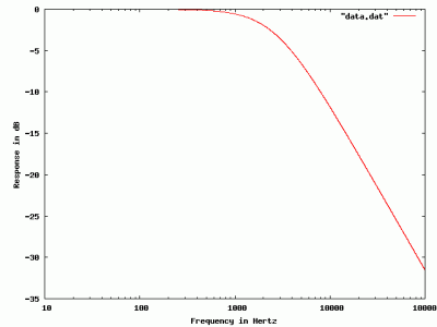
If you take the data that gets printed out here and graph it, you get the following:

I built the same circuit in LTSpice just to check my understanding, and the graph appears identical. If you search through the data to find the place where the response drops to -3db, you find it occurs around 2650 Hz. The traditional formula for filter bandwidth is

[latex]F = \frac{1}{2 \pi R C}[/latex]

which when you plug in the values I chose, you end up with 2653.9 (which is pretty good agreement).

Addendum: This filter works best when the input impedance is very low (compared to the 600 ohms that we chose for the input resistor [latex]R[/latex]) and where the load impedance [latex]Rload[/latex] (here purely resistive, but it could also be complex) is high. If the load were low (Rload was comparable or less than than R) then the losses would be higher. (Ignore the capacitor. If Rload is small compared to R, then the voltage, even at DC, is already divided down to a lower value, this shifts the entire curve downward).

Addendum²: I wrote this hastily. If it doesn’t make sense, or people have suggestions, don’t hesitate to add them in the comments below.

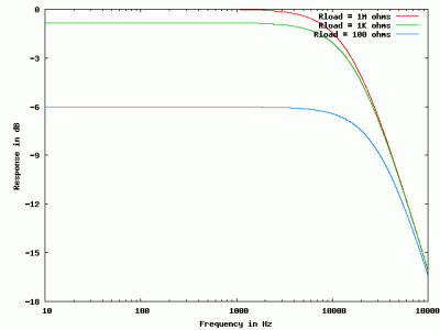
Addendum³: Atdiy asked me to run some simulations showing how the load [latex]Rload[/latex] changes the output to demonstrate loss. Here, I kept [latex]R = 100[/latex], but varied [latex]Rload[/latex] from 1M ohms, to 1Kohms, and then down to just 100ohms. You can see the entire curve moves down, with only 100 ohms of load resistance, the voltage is -6db (multiplied by 0.25) even at DC).

Addendum⁴: Atidy has started her series on filter design, which includes a qualitative description of how these filters work that you might find easier to understand. Check it out here.
.