This week began with a visit from Pat Hanrahan, currently a professor at Stanford and formerly at Princeton, where I was lucky enough to meet him. He came by to talk about probabilistic programming languages, which are an interesting topic that he and his students have made some interesting progress in solving difficult problems. I don’t have much to say about it, except that it seemed very cool in a way which I’ve come to expect from Pat: he has a tendency to find interesting cross disciplinary connections and exploit them in ways that seem remarkable. I haven’t had much time this week to think about his stuff more, but he did mention this website which gives examples of probabilistic computation and cognition, which seemed pretty cool. I’m mostly bookmarking it for later consumption.
Category Archives: Computer Graphics
Deconstructing the Classic Atari Game: Star Raiders
Gasp, I know. It’s been some time since I posted here. A combination of life and work events have conspired to sap me of my usual exuberant energy for the nerdy, geeky pointless topics that I usually like to post about here. But nerdy, geeky, pointless endeavors do continue (even if at a reduced pace) so I thought I’d post about one here that I’ve killed a few hours on.
I have fallen back into thinking about retrocomputing, not so much out of a sense of nostalgia, but because I was trying to understand the complex path that connected a 12 year old boy growing up in Oregon to the one who now exists. I think in no small part, I can draw it back to this game:
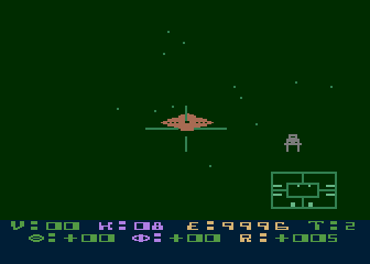
The classic 1979 Atari game Star Raiders. I’m pretty sure it was the second cartridge I bought for my Atari 400, right after Atari BASIC. Within it’s 8K boundaries, a first person space simulation was created. Not the boring, type “LRS” to get long range scan respresented in crude ASCII charts, but instead a visceral battle against the Zylon menace.
As much as I liked the game (and have played it a few times in the last few days, it still pretty much holds up) it also inspired me back then to learn how such highly interactive, real time games could be written. I got a copy of De Re Atari, and worked on learning about machine language programming, and how to manipulate POKEY and ANTIC to do my bidding. I used to say that the Atari was the last computer that I understood completely. Perhaps that was a little bit of bragging, combined with the humble realization that modern computers were far more of a black box than I felt I could understand.
But in the last couple of weeks, I thought to myself, “there must be some good programming hidden away in that 8K.” The scientist in me recognizes beauty not just in the final form of the organism, but in its constituent parts. So, I decided to see if I could take the raw ROM image of Star Raiders, and turn it back into an annotated chunk of source code. In theory, you could use this to make changes (I hesitate to say “fixes”, because it’s so brilliant) but really, it was just so I can learn something about how it works.
Luckily for me, modern tools have made this much simpler. I have a Linux box far more powerful than any computer I could have dreamed of back in the day, and retrocomputing pioneers have traveled this path already, and left tools that I could use along the way. I decided to use cc65, a freeware C compiler suite that can generate code for a variety of classic 6502 based systems. It includes da65, a disassembler that will take an “info” file which describes where the code starts and some machine specific labels, and then tries to disassemble the ROM back into assembly code. It more of less seems to default to the idea that the ROM is entirely code, and only inserts “.byte” assembly instructions when it can’t find a valid instruction at a particular location. By beginning at the known jump address, you can follow code and find areas where data instructions access tables and the like, and then use the .info file to describe block those out, slowly converging to more or less legible code. For instance, the decoded code that starts the cartridge looks like this:
; ----------------------------------------------------------------------------
CARTBOOT:
        lda     #$00                            ; A14A A9 00                    ..
        sta     SKCTL                           ; A14C 8D 0F D2                 ...
        sta     $66                             ; A14F 85 66                    .f
        sta     $62                             ; A151 85 62                    .b
        sta     $63                             ; A153 85 63                    .c
        lda     #$03                            ; A155 A9 03                    ..
        sta     SKCTL                           ; A157 8D 0F D2                 ...
LA15A:  ldy     #$2F                            ; A15A A0 2F                    ./
LA15C:  lda     #$FF                            ; A15C A9 FF                    ..
LA15E:  sty     $65                             ; A15E 84 65                    .e
        sta     $64                             ; A160 85 64                    .d
        lda     #$00                            ; A162 A9 00                    ..
        tax                                     ; A164 AA                       .
LA165:  sta     HPOSP0,x                        ; A165 9D 00 D0                 ...
        sta     DMACTL,x                        ; A168 9D 00 D4                 ...
        cpx     #$0F                            ; A16B E0 0F                    ..
        bcs     LA172                           ; A16D B0 03                    ..
        sta     AUDF1,x                         ; A16F 9D 00 D2                 ...
LA172:  sta     PORTA,x                         ; A172 9D 00 D3                 ...
        sta     a:$67,x                         ; A175 9D 67 00                 .g.
        inx                                     ; A178 E8                       .
        bne     LA165                           ; A179 D0 EA                    ..
        dex                                     ; A17B CA                       .
        txs                                     ; A17C 9A                       .
        cld                                     ; A17D D8                       .
        lda     #$02                            ; A17E A9 02                    ..
        jsr     LAE0F
Seems like typical “begin the program” kind of stuff, the loop around LA165 is basically zeroing out a lot of I/O ports which control player missile graphic and audio, as well as lots of zero page memory starting around address $67. Not too exciting, but it gets you started.
A bit of poking (and review of old Atari programming manuals) made me realize that the system sets up the player missile graphics to be based from address zero. This means that the buffers for the player 0 will start at $400, for player 1 at $500, etc… Some further poking indicates that the display list (the list of ANTIC instructions that builds the display) begins at $280. I located a couple of data tables that contained a list of strings used in the game (with the first character in each having the high bit set). I located a fragment of a display list in ROM. I wrote a python program to generate a graphical version of each instruction (1s displayed as X’s, 0s as spaces) to see if I could locate some of the bit patterns from the game. This revealed that some font characters were defined starting right at the beginning of the ROM (mapped to address $A00) as well as the bit patterns for the TIE fighters, asteroids, etc…) in a variety of sizes:
B9B0:  X X
    :
    :X      X
    :X      X
    :X      X
    :X      X
    :X XXXX X
    :XXXXXXXX
B9B8:XXXXXXXX
    :X XXXX Xh
    :X      X
    :X      X
    :X      X
    :X      X
    :X     X
    :X     X
B9C0:X XXX X
    :XXXXXXX
    :XXXXXXX
    :X XXX X
    :X     X
    :X     X
That was helpful. But then progress began to slow a bit, and I wondered what other tools I could use. Back when I was teaching myself Atari 2600 programming, I found the Stella simulator to be absolutely key: it had an awesome single step debugger that I used to work out many a difficult chunk of code. Without any real research, I settled on using the atari800 simulator from sourceforge. A bit of digging uncovered that hitting F8 dropped you into a monitor. Not as sophisticated as the Stella one, but still quite helpful. For instance, if you type “DLIST”, you can get the currently active display list. During the “attract mode” of the game, you can break and find that the current display list is:
0280: 2x 8 BLANK
0282: LMS 1000 MODE D
0285: 10x MODE D
028F: 4 BLANK
0290: LMS 0D1F MODE 6
0293: LMS 12A8 MODE D
0296: 81x MODE D
02E7: JVB 0280
This is pretty helpful (although it’s probably gobblety-gook to most readers). Reading from top to bottom, it says that the display has 16 scanlines which are blank, then starts rendering with mode D (which is a 160 pixel resolution, 4 color mode, where each dot is 2 scanlines high). The LMS indicates that the graphics memory will start at $1000. There are a few more lines like that, then some blank lines followed by a mode 6 line (which is a 20 character display, 8 scanlines high). Then some more lines of Mode D (resetting the memory buffer to the appropriate address). The mode 6 line draws characters from the buffer beginning at $0D1F, which I had not identified in code anywhere. That presented a clue to me, enabling me to spot other useful chunks of code.
I’ll keep plodding away at this, it is kind of like working on a crossword puzzle. Each little bit you uncover allows you to understand more. Stay tuned.
Simple code implementing the SmoothLifeL cellular automata…
Without further ado… if you want code to implement this:
You can download this this zip file. Do with it what you will.
Fourier Volume Rendering
Three years ago, I wrote a short post about volume rendering. I always meant to follow up, because I finally sorted out the problems with generating multiple, overlapping images. Here’s a new video generated with the improved code:
Fourier volume rendering is less flexible than raytracing, but it does have certain computational advantages, most notably in that you can generate images in less than O(n^3) time, which is the typical bound for conventional raytracing. It also has some applications in light field refocusing applications. But overall, I still thing that raytracing has a number of advantages. Perhaps that would make a good first serious Go program? I’ll ponder it more.
More Wisdom on LEDs…
More important help for the budding young electronics designer:
https://twitter.com/#!/EMSL/status/144546376624250880
Note: this also works in computer graphics quite well. Just specify a negative intensity for the light value.
Making some wallpaper with the sum of cosines…
I was inspired by some Haskell code written by keegan, so I had to write a version of it in C. I didn’t do any animation, but I did have a lot of fun playing around with the parameters. For instance, check out the code, and how changing the value of N from 5, 7, and 19 generates interesting and cool patterns.
[sourcecode lang=”cpp”]
#include <stdio.h>
#include <stdlib.h>
#include <math.h>
#include <assert.h>
/*
* quasi.c
*
* Some code, inspired by keegan @
* http://mainisusuallyafunction.blogspot.com/2011/10/quasicrystals-as-sums-of-waves-in-plane.html
* but presented without any further explanation.
*/
#define N (19)
#define XSIZE (1280)
#define YSIZE (720)
#define SCALE (0.2)
double x[N], y[N], ph[N] ;
double image[YSIZE][XSIZE] ;
int
main()
{
int i, j, k ;
for (i=0; i<N; i++) {
x[i] = cos(2.0 * M_PI * i / (double) N) ;
y[i] = sin(2.0 * M_PI * i / (double) N) ;
ph[i] = 0.0 ;
}
for (j=0; j<YSIZE; j++) {
for (i=0; i<XSIZE; i++) {
image[j][i] = 0. ;
for (k=0; k<N; k++) {
double d = (x[k] * (i – XSIZE / 2.) + y[k] * (j – YSIZE / 2.) + ph[k]) * SCALE ;
image[j][i] += (1.0 + cos(d)) / 2. ;
}
int t = (int) floor(image[j][i]) ;
assert(t >= 0.) ;
double v = image[j][i] – t ;
if (t % 2 == 1) v = 1. – v ;
image[j][i] = v ;
}
}
printf("P5\n%d %d\n%d\n", XSIZE, YSIZE, 255) ;
for (j=0; j<YSIZE; j++)
for (i=0; i<XSIZE; i++)
putchar(255. * image[j][i]) ;
return 0 ;
}
[/sourcecode]


Cool stuff!
Watermarking and titling with ffmpeg and other open source tools…
I’ve received two requests for information about my “video production pipeline”, such as it is. As you can tell by my videos, I am shooting with pretty ugly hardware, in a pretty ugly way, with minimal (read “no”) editing. But I did figure out a pretty nice way to add some watermarks and overlays to my videos using open source tools like ffmpeg, and thought that it might be worth documenting here (at least so I don’t forget how to do it myself).
First of all, I’m using an old Kodak Zi6 that I got for a good price off woot.com. It shoots at 1280x720p, which is a nominally a widescreen HD format. But since ultimately I am going to target YouTube, and because the video quality isn’t all that astounding anyway, I have chosen in all my most recent videos to target a 480 line format, which (assuming 16:9) aspect ratio means that I need tor resize my videos down to 854×480. The Zi6 saves in a Quicktime container format, using h264 video and AAC audio at 8Mbps and 128kbps respectively.
For general mucking around with video, I like to use my favorite Swiss army knife: ffmpeg. It reads and writes a ton of formats, and has a nifty set of features that help in titling. You can try installing it from whatever binary repository you like, but I usually find out that I need to rebuild it to include some option that the makers of the binary repository didn’t think to add. Luckily, it’s not really that hard to build: you can follow the instructions to get a current source tree, and then it’s simply a matter of building it with the needed options. If you run ffmpeg by itself, it will tell you what the configuration options it used for compilation. For my own compile, I used these options:
--enable-libvpx --enable-gpl --enable-nonfree --enable-libx264 --enable-libtheora --enable-libvorbis
--enable-libfaac --enable-libfreetype --enable-frei0r --enable-libmp3lame
I enabled libvpx, libvorbis and libtheora for experimenting with webm and related codecs. I added libx264 and libfaac so I could do MPEG4, mp3lame so I could encode to mp3 format audio, most important for this example, libfreetype so it would build video filters that could overlay text onto my video. If you compile ffmpeg with these options, you should be compatible with what I am doing here.
It wouldn’t be hard to just type a quick command line to resize and re-encode the video, but I’m after something a bit more complicated here. My pipeline resizes, removes noise, does a fade in, and then adds text over the bottom of the screen that contains the video title, my contact information, and a Creative Commons banner so that people know how they can reuse the video. To do this, I need to make use of the libavfilter features of ffmpeg. Without further ado, here’s the command line I used for a recent video:
[sourcecode lang=”sh”]
#!/bin/sh
./ffmpeg -y -i ../Zi6_4370.MOV -sameq -aspect 16:9 -vf "scale=854:480, fade=in:0:30, hqdn3d [xxx]; color=0x33669955:854×64 [yyy] ; [xxx] [yyy] overlay=0:416, drawtext=textfile=hdr:fontfile=/usr/share/fonts/truetype/ttf-dejavu/DejaVuSerif-Bold.ttf:x=10:y=432:fontsize=16:fontcolor=white [xxx] ; movie=88×31.png [yyy]; [xxx] [yyy] overlay=W-w-10:H-h-16" microfm.mp4
[/sourcecode]
So, what does all this do? Well, walking through the command: -y says to go ahead and overwrite the output file. -i specifies the input file to be the raw footage that I transferred from my Zi6. I specified -sameq to keep the quality level the same for the output:: you might want to specify an audio and video bitrate separately here, but I figure retaining the original quality for upload to YouTube is a good thing. I am shooting 16:9, so I specify the aspect ratio with the next argument.
Then comes the real magic: the -vf argument specifies a rather long command string. You can think of it as a series of chains, separated by semicolons. Each command in the chain is separated by commas. Inputs and outputs are specified by names appearing inside square brackets. Read the rather terse and difficult documentation if you want to understand more, but it’s not too hard to walk through what the chains do. From ‘scale” to the first semicolon, the input video (implicit input to the filter chain) we resize the video to the desired output size, fade in from black over the first 30 frames, and then run the high quality 3d denoiser, storing the result in register xxx. The next command creates a semi-transparent background color card which is 64 pixels high and the full width of the video, storing it in y. The next command takes the resized video xxx, and the color card yyy, and overlays the color at the bottom. We could store that in a new register, but instead we simply chain on a drawtext command. It specifies an x, y, and fontfile, as well as a file “hdr” which contains the text that we want to insert. For this video, that file looks like:
The (too simple) Micro FM transmitter on a breadboard
https://brainwagon.org | @brainwagon | mailto:brainwagon@gmail.com
The command then stores the output back in the register [xxx]. The next command reads a simple png file of the Creative Commons license and makes it available as a movie in register yyy. In this case, it’s just a simple .png, but you could use an animated file if you’d rather. The last command then takes xxx and yyy and overlays them so that the copyright appears in the right place.
And that’s it! To process my video, I just download from the camera to my linux box, change the title information in the file “hdr”, and then run the command. When it is done, I’m ready to upload the file to YouTube.
A couple of improvements I have yet to add to my usual pipeline: I don’t really like the edge of the transparent color block: it would be nicer to use a gradient. I couldn’t figure out how to synthesize one in ffmpeg, but it isn’t hard if you have something like the netpbm utilities:
[sourcecode lang=”sh”]
#!/bin/sh
pamgradient black black rgb:80/80/80 rgb:80/80/80 854 16 | pamtopnm > grad1.pgm
ppmmake rgb:80/80/80 854 48 | ppmtopgm > grad2.pgm
pnmcat -tb grad1.pgm grad2.pgm > alpha.pgm
ppmmake rgb:33/66/99 854 64 > color.ppm
pnmtopng -force -alpha alpha.pgm color.ppm > mix.png
[/sourcecode]
Running this command builds a file called ‘mix.png’, which you can read in using the movie node in the avfilter chain, just as I did for the Creative Commons logo. Here’s an example:
If I were a real genius, I’d merge this whole thing into a little python script that could also manage the uploading to YouTube.
If this is any help to you, or you have refinements to the basic idea that you’d like to share, be sure to add your comments or links below!
Code from the Past: a tiny real time raytracer from 2000
Back in 2000, I was intrigued by the various demos that I saw which attempted to implement real time raytracing. I wondered just what could be done with the computers I had on hand, without using any real tricks, but just a straightforward implementation of ray/sphere and ray/patch intersection. As I recall, I got two or three frames a second back then. I dusted off this code, and recompiled it for my MacBook (it uses OpenGL/GLUT, so it should be reasonably portable) and now it actually runs pretty reasonably. The code isn’t completely horrific, and might be of some use to someone as an example. It’s not clever, just straightforward and relatively easy to understand.
RTRT3, a tiny realtime raytracer

Addendum: I recompiled this on some of our spiffy machines at work, and immediately encountered a bug: there is nothing really to prevent infinite recursion. It’s possible (especially when the sphere and plane are touching) for a ray to get “stuck” between the sphere and plane. The simplest cure is to just keep track of how deep the recursion is by passing a “level” variable down through the intersect routines, and return FALSE for any intersection which is “too deep” (say, beyond six reflections deep). When modified thusly, I get about 96 FPS on my current HP desktop machine, running on one core. It has 12, incidently.
Cool Hack O’ Day: real pixel coding
The problem with working some place with lots of intelligent people is that it is increasingly hard to maintain one’s sense of superiority. Today, I tip my hat to Inigo. He has a very cool demo here, where he creates a program by creating and editing a small image in photoshop, saving it as a raw image file, and then renaming it to a .COM file and running it. It’s a testament to how clever, sneaky, and small programs can be.
Thanks to Jeri reposting this link on twitter, I’m getting lots of hits. Thanks Jeri. But be sure to visit Inigo’s original post to read more about this cool hack:
el trastero » Blog Archive » real pixel coding.
Hershey Vector Fonts
 Nearly thirty years ago, I remember hacking together some simple code to display graphics on a WYSE 35 terminal. The terminals supported the TEK 4014 graphics commands to draw vectors, and I found the original “Hershey Fonts”, created by A.V. Hershey at the U.S. National Bureau of Standards, and placed in the public domain.
I’ve come full circle it appears. Having some vector fonts for my oscilloscope experimentation would be really handy. I had nearly forgotten them, until my friend Tom reminded me of them. Digging around found Paul Bourke’s cool web site which archived a lot of this information, and provided a quick, cogent explanation of the data:
The full Hershey set is supplied here for Roman
via Hershey Vector Font.
Somewhere… over the (simulated) rainbow revisited…
A couple of months ago, I did some simple simulations of light refracting through raindrops in a hope to understand the details of precisely how rainbows form. The graphs I produced were kind of boring, but they did illustrate a few interesting features of rainbows: namely, the double rainbow, and the formation of Alexander’s band, the region of relatively dark sky between the two arcs.
But the pictures were kind of boring.
So, today I finally got the simulation working, did a trivial monte carlo simulation tossing fifty million rays or so, and then generated a picture by converting the spectral colors to sRGB. Et voila!

Horribly inefficient really, but satisfying result.
Addendum: In comparing the results to actual photographs of double rainbows, it seems like my pictures are scaled somewhat strangely (the distance between the arcs seems large compared to the radius). I suspect this is mostly due to the linear projection that I used and the very wide field (the field of view of the camera is nearly 100 degrees, which compresses the center and expands the outside. I’ll have to make some narrower field pictures tomorrow when my mind can handle the math, I’ve reached my limit tonight.
On random numbers…
While hacking a small program today, I encountered something that I hadn’t seen in a while, so I thought I’d blog it:
My random number generator failed me!
I was implementing a little test program to generate some random terrain. The idea was pretty simple: initialize a square array to be all zero height. Set your position to be the middle of the array, then iterate by dropping a block in the current square, then moving to a randomly chosen neighbor. Keep doing this until you place as many blocks asu like (if you wander off the edge, I wrapped around to the other side), and you are mostly done (well, you can do some post processing/erosion/filtering).
When I ran my program, it generated some nice looking islands, but as I kept iterating more and more, it kept making the existing peaks higher and higher, but never wandered away from where it began, leaving many gaps with no blocks at all. This isn’t supposed to happen in random walks: in the limit, the random walk should visit each square on the infinite grid (!) infinitely often (at least for grids of dimension two or less).
A moment’s clear thought suggeseted what the problem was. I was picking one of the four directions to go in the least complicated way imaginable:
[sourcecode lang=”C”]
dir = lrand48() & 3 ;
[/sourcecode]
In other words, I extracted just the lowest bits of the lrand48() call, and used them as an index into the four directions. But it dawned on me that the low order bits of the lrand48() all aren’t really all that random. It’s not really hard to see why in retrospect: lrand48() and the like use a linear congruential generator, and they have notoriously bad performance in their low bits. Had I used the higher bits, I probably would never have noticed, but instead I just shifted to using the Mersenne Twister code that I had lying around. And, it works much better, the blocks nicely stack up over the entire 5122 array, into pleasing piles.
Here’s one of my new test scenes:

Much better.
Somewhere… over the (simulated) rainbow…
A few days back, I simulated how light propagated in a single drop of water, but with a number of problems. First of all, it didn’t simulate the Fresnel equations, which describe how light is reflected and refracted at the interface between two media. This meant that in my simple model, no light is actually subject to total internal reflection, and no light was scattered back in the direction that the light originated. This is an important effect: without it, you cannot see rainbows. It also assumed a single index of refraction, so we couldn’t see how the reflection and refraction change as a function of wavelength.
So, I decided to fix both problems, and run a simulation to see if I could capture some interesting features of rainbows by direct simulation.
To keep you interested (if possible), I’ll merely give the picture, then explain it. (Click on it to view it full size).

Simulated rainbow reflection, light enters from left, goes to right
It’s hard to see the detail in the area of interest, so here’s a better version, zoomed in (click to view bigger):

This describes the distribution of light in each outgoing direction, assuming light coming in from the left. There are four different plots, ranging from the shortest wavelength (4047 Angstroms, or deep violet) to the longest (7065 Angstroms, or deep red). (Sadly, there isn’t any correlation between the plot color and the wavelength, you have to look at the legend to interpret things properly.) I got these plots by determining the index of water at each wavelength, and then simulating via Monte Carlo techniques the resulting outgoing distribution by tossing 10 million simulated photons at the drop. At each surface interaction, it determines what the ratio of reflected to refracted light could be, and then take one path or the other based upon a weighted coin flip. The final outgoing directions are binned, and we take the log of the count in each bin to produce the distance from the center in the polar plot.
This plot isn’t the most pretty thing you’ll ever see, but you’ll actually find a number of interesting things. First of all, you’ll see that there are two rainbows represented. The inner one is the brighter, and the outer one is significantly dimmer (you might estimate that it contains 1/10 as much energy, since it appears about 1 unit lower and I used log based 10). The inner bow has violet at the inner side, and red at the outer side while the outer bow is reversed (red on the inner radius and violet on the outer radius). There is also a distinct lack of light between the two bows. The amount of light reflected in between the two bows is less than that scattered outside them. This is a phenomenon called “Alexander’s band”.
I thought this was a fun experiment. I could work a bit harder and actually produce the appropriate colors and intensities by some more computer graphics magic. Perhaps that will wait for some other day.
Drawing “circles” ala Marvin Minsky…
In my re-reading of Levy’s book Hackers, I was reminded of an interesting bit of programming lore regarding an early display hack that Marvin Minsky did for circle drawing. It’s an interesting hack because the lore was that it was originally coded by mistake, and yet the result proved to be both interesting and even useful. I first learned of this years ago when Blinn did an article on different ways to draw a circle, but also learned that it was part of the MIT AI memo called “HAKMEM”. Here’s the basic idea:
One way that you can draw a circle is to take some point x, y on the circle, and then generate new points by rotating them around the center (let’s say that’s the origin for ease) and connecting them with lines. If you have a basic understanding of matrix math, it looks like this:
/ x' \   /  cos theta  sin theta \ / x \
|    | = |                       | |   |
\ y' /   \ - sin theta cos theta / \ y /
(I should learn how to use MathML, but you hopefully get the idea). The matrix with the cosine and sine terms in it is a rotation matrix which rotates a point around by the angle theta. Apparently Minsky tried to simplify this by noting that cos(theta) is very nearly one for small theta, and that sin(theta) can be approximated by theta (we can get this by truncating the Taylor series for both). Therefore, he thought that (I’m guessing here, but it seems logical) that we could simplify this as:
/ x' \   /   1  eps \ / x \
|    | = |          | |   |
\ y' /   \ -eps  1  / \ y /
Okay, it’s pretty obvious that this seems like a bad idea. For one thing, the “rotation” matrix isn’t a pure rotation. It’s determinant is 1 – eps^2 1 + eps^2, which means that points which are mapped move slowly toward away from the origin. Nevertheless, Minsky apparently thought that it might be interesting, so he went ahead an implemented the program. I’ll express it here is pseudo-code:
newx = oldx - eps * oldy
newy = oldy + eps * newx
Note: this program is “buggy”. The second line should (for some definition of should) read “oldy + eps * oldx“, but Minsky got it wrong. Interestingly though, this “bug” has an interesting side effect: it draws circles! If eps is a power of 2, you can even implement the entire thing in integer arithmetic, and you don’t need square roots or floating point or anything. Here’s an example of it drawing a circle of radius 1024:

Well, there is a catch: it doesn’t really draw circles. It draws ellipses. But it’s still a very interesting bit of code. The first thing to note is that if you actually write down the transformation matrix that the “wrong” equations implement, the determinant is one. That helps explain why the point doesn’t spiral in. But there is another odd thing: if you implement this in integer based arithmetic, it’s eventually periodic (it doesn’t go out of control, all the round off errors eventually cancel out, and you return to the same point again and again and again). In HAKMEM, Schroeppel proclaims that the reason for the algorithm’s stability was unclear. He notes that there are a finite number of distinct radii, which indicates that perhaps the iterative process will always eventually fill in the “band” of valid radii, but the details of that seem unclear to me as well. I’ll have to ponder it some more.
Addendum: The real reason I was looking at this was because the chapter in Hackers which talks about Spacewar! also talks about the Minskytron whose official name was TRI-POS. It apparently uses some of this idea to draw curves in an interesting way. HAKMEM item #153 also suggests an interesting display hack:
ITEM 153 (Minsky):
To portray a 3-dimensional solid on a 2-dimensional display, we can use a single circle algorithm to compute orbits for the corners to follow. The (positive or negative) radius of each orbit is determined by the distance (forward or backward) from some origin to that corner. The solid will appear to wobble rigidly about the origin, instead of simply rotating.
Might be interesting to implement.
Addendum2: I goofed up the determinant above, it should be 1 + eps^2, not 1-eps^2. Corrected.
Simple, reliable 2.5D photography
I’ve been interested in techniques where amateurs can digitize images and models for quite a bit. This website percolated to the top during today’s relaxing web browsing: it’s pretty spiffy, and is interesting on a couple of fronts, not the least of which is that the author designed the gearbox for tracking a laser using a CAD program which drove a CNC mill so that the parts could be cast. Very slick.