Category Archives: Math

On calculators, Space Invaders and Binary Coded Decimal Arithmetic…

A couple days ago, one of my Twitter or Facebook friends (sadly, I forgot who, comment if it was you, and I’ll give you credit) pointed out this awesome page:

Reversing Sinclair’s amazing 1974 calculator hack – half the ROM of the HP-35

It documented an interesting calculator made by Sinclair in the 1970s. It is an awesome hack that was used to create a full scientific calculator with logarithms and trigonometric functions out of an inexpensive chip from TI which could (only barely) do add, subtract, multiply and divide. The page’s author, Ken Shirriff, wrote a nifty little simulator for the calculator that runs in the browser. Very cute. It got me thinking about the bizarre little chip that was at the center of this device.

I’m kind of back in an emulator kick. I recently had dusted off my code that I had started for emulating the 8080 processor. I had originally wanted to implement a version of CP/M, but I remembered that the 1978 game Space Invaders was also based upon the 8080. It wasn’t hard to find a ROM file for it, and with a little bit of hacking, research and debugging, I had my own version of Space Invaders written in C and using SDL2, running on my Mac laptop.

Screen Shot 2015-09-16 at 12.46.01 PM

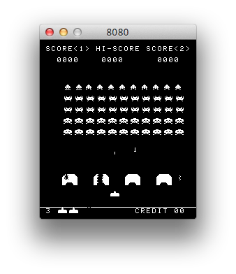
Fun stuff.  The sound is a little crude: most of the sound in the original game was generated by a series of discrete circuits which you can find on this page archived via the Wayback Machine. I briefly played around with simulating some of the sounds using LTSpice based upon these circuits (it appears to work fairly well), but I haven’t got that fully integrated into my simulator yet. For now, it just queues up some recorded sounds and plays them at the appropriate time. Everything is currently working except for the classic “thump… thump…” of their marching. I’ll get that working sometime soon.

Anyway, back to calculators. One thing on Ken’s page kind of made me think: he mentioned that the HP-35 had taken two years, twenty engineers, and a million dollars to develop. Mind you, the HP-35 was pretty revolutionary for its time. But I thought to myself “isn’t a calculator an easy hobby project now?”

After all, I had assembled a KIM-Uno, Oscar’s awesome little $10 board that emulates the KIM-1 microcomputer:

In fact, the KIM-Uno implements a floating point calculator as well. It’s brains are just an ordinary Arduino Pro Mini wired on the back. Arduino Pro Minis can be had for less than $3 from China. Could I make a fun little calculator using that as the basis?

My mind is obviously skipping around a lot at this point.

Of course, a bit more googling revealed that someone had done something very similar using the MSP430 chips from (appropriately enough, also manufactured by Texas Instruments). Check out the build thread here.. It’s pretty nifty, and uses a coin cell to drive it, as well as some very classic looking “bubble LED displays”, which you can get from Sparkfun. Pretty cool.

Anyway…

For fun, I thought it might be fun to write some routines to do binary coded decimal arithmetic. My last real experience with it was on the 6502 decades ago, and I had never done anything very sophisticated with it. I understood the basic ideas, but I needed some refresher, and was wondering what kind of bit twiddling hacks could be used to implement the basic operations. Luckily, I stumbled onto Douglas Jones’ page on implementing BCD arithmetic, which is just what the doctor ordered. He pointed out some cool tricks and wrinkles associated with various bits of padding and the like. I thought I’d code up a simple set of routines that stored 8 BCD digits in a standard 32 bit integer. His page didn’t include multiplication or division. Multiplication was simple enough to do (at least in this slightly crazy “repeated addition” way) but I’ll have to work a bit harder to make division work. I’m not sure I really know the proper way to handle overflow and the sign bits (my multiplication currently multiplies two 8 digit numbers, and only returns the low 8 digits of the result). But.. it seems to work.

And since I haven’t been posting stuff to my blog lately, this is an attempt to get back to it.

Without further ado, here is some code:

[sourcecode lang=”C”]
/*
* A simple implementation of the ideas/algorithms in
* http://homepage.cs.uiowa.edu/~jones/bcd/bcd.html
*
* Written with the idea of potentially doing a simple calculator that
* uses BCD arithmetic.
*/

#include <stdio.h>
#include <stdint.h>
#include <inttypes.h>

typedef uint32_t bcd8 ; /* 8 digits packed bcd */

int
valid(bcd8 a)
{
bcd8 t1, t2, t3, t4 ;
t1 = a + 0x06666666 ;
t2 = a ^ 0x06666666 ;
t3 = t1 ^ t2 ;
t4 = t3 & 0x111111110 ;
return t4 ? 0 : 1 ;
}

bcd8
add(bcd8 a, bcd8 b)
{
bcd8 t1, t2, t3, t4, t5, t6 ;

t1 = a + 0x06666666 ;
t2 = t1 + b ;
t3 = t1 ^ b ;
t4 = t2 ^ t3 ;
t5 = ~t4 & 0x11111110 ;
t6 = (t5 >> 2) | (t5 >> 3) ;
return t2 – t6 ;
}

bcd8
tencomp(bcd8 a)
{
bcd8 t1 ;

t1 = 0xF9999999 – a ;
return add(t1, 0x00000001) ;
}

bcd8
sub(bcd8 a, bcd8 b)
{
return add(a, tencomp(b)) ;
}

bcd8
mult(bcd8 a, bcd8 b)
{
bcd8 result = 0 ;
bcd8 tmp = a ;
bcd8 digit ;
int i, j ;

for (i=0; i<8; i++) {

digit = b & 0xF ;
b >>= 4 ;

for (j=0; j<digit; j++)
result = add(result, tmp) ;

tmp <<= 4 ;
}
return result ;
}

int
main(int argc, char *argv[])
{
bcd8 t = 0x00009134 ;
bcd8 u = 0x00005147 ;
bcd8 r ;

r = mult(t, u) ;
printf("%X * %X = %X\n", t, u, r) ;
}
[/sourcecode]

I’ll have to play around with this some more. It shouldn’t be hard to move code like this to run on the Arduino Pro Mini, and drive 3 bubble displays (yielding 11 digits plus a sign bit) of precision. And I may not use this 8 digits packed into 32 bit format: since I want 12 digits, maybe packing only 4 digits into a 32 bit word would work out better.

Anyway, it’s all kind of fun to think about the clanking clockwork that lived inside these primitive machines.

I’ll try to post more often soon.

One dimensional cellular automata code in Python..

Inspired by the KnitYak Kickstarter, I thought I would code up a simple Python program that could generate the same sort of patterns that are used in the scarves in the video. If you want to learn more about the mathematical theory of these cellular automata, google for keywords like “1D” “cellular automata” and “steve wolfram”. Without much further explanation, here is the code:

[sourcecode lang=”python”]
#!/usr/bin/env python

# __
# ___ __ __ _ _ _ / _|
# (_-</ _/ _` | ‘_| _|
# /__/\__\__,_|_| |_|
#
# Inspired by the KnitYak Kickstarter, which offers
# mathematical scarves whose patterns are algorithmically
# generated, I thought it would be good to dust off my old
# knowledge and generate the same sort of patterns using
# Python. The patterns are simply printed using ASCII,
# but the code could be adapted to output in other forms
# easily.
#
# Written by Mark VandeWettering
#

import sys
import random

WIDTH=79 # How wide is the pattern?

w = WIDTH * [0] # create the current generation
nw = WIDTH * [0] # and the next generation
w[WIDTH/2] = 1 # populate with a single one

# or alternatively, you can populate it with a random
# initial configuration. If you want to start with
# just a single one, comment the next two lines out.

#for i in range(WIDTH):
# w[i] = random.randint(0, 1)

# How wide is the neighborhood of cells that are
# examined? The traditional Wolfram 1D cellular
# automata uses a neighborhood of 3…

NEIGHBORHOOD=3

# rtab is space for the rule table. It maps all
# numbers from [0, 2**NEIGHBORHOOD) to either a 0 or 1.
rtab = (2**NEIGHBORHOOD) * [0]

# The "rule" is a number which is used to populate
# rtab. The number is in the range [0, 2**(2**NEIGHBORHOOD))
# Many rules generate uninteresting patterns, but some
# like 30 generate interesting, aperiodic patterns.
rule = 30

# This fills in the table…
for i in range(2**NEIGHBORHOOD):
if ((2**i) & rule) != 0:
rtab[i] = 1

def dump(r):
for x in r:
if x == 1:
sys.stdout.write(‘X’)
else:
sys.stdout.write(‘ ‘)
sys.stdout.write(‘\n’)

# and generates 100 lines…

for y in range(100):
dump(w)
for x in range(WIDTH):
sum = 0
for d in range(NEIGHBORHOOD):
sum = sum + (2**d) * w[(x+d+WIDTH – NEIGHBORHOOD/2) % WIDTH]
nw[x] = rtab[sum]
w, nw = nw, w
[/sourcecode]

The pattern this generates with these settings follows. Try adjusting rule to other numbers up to 255 to generate other patterns. Lots will be boring, but some will be pretty interesting.

                                                                               
                                       X                                       
                                      XXX                                      
                                     X  XX                                     
                                    XXXX XX                                    
                                   X   X  XX                                   
                                  XXX XXXX XX                                  
                                 X  X    X  XX                                 
                                XXXXXX  XXXX XX                                
                               X     XXX   X  XX                               
                              XXX   X  XX XXXX XX                              
                             X  XX XXXX X    X  XX                             
                            XXXX X    X XX  XXXX XX                            
                           X   X XX  XX  XXX   X  XX                           
                          XXX XX  XXX XXX  XX XXXX XX                          
                         X  X  XXX  X   XXX X    X  XX                         
                        XXXXXXX  XXXXX X  X XX  XXXX XX                        
                       X      XXX    X XXXX  XXX   X  XX                       
                      XXX    X  XX  XX    XXX  XX XXXX XX                      
                     X  XX  XXXX XXX XX  X  XXX X    X  XX                     
                    XXXX XXX   X   X  XXXXXX  X XX  XXXX XX                    
                   X   X   XX XXX XXXX     XXXX  XXX   X  XX                   
                  XXX XXX X X   X    XX   X   XXX  XX XXXX XX                  
                 X  X   X X XX XXX  X XX XXX X  XXX X    X  XX                 
                XXXXXX XX X  X   XXXX  X   X XXX  X XX  XXXX XX                
               X     X  X XXXXX X   XXXXX XX   XXXX  XXX   X  XX               
              XXX   XXXXX     X XX X    X  XX X   XXX  XX XXXX XX              
             X  XX X    XX   XX  X XX  XXXX X XX X  XXX X    X  XX             
            XXXX X XX  X XX X XXXX  XXX   X X  X XXX  X XX  XXXX XX            
           X   X X  XXXX  X X    XXX  XX XX XXXX   XXXX  XXX   X  XX           
          XXX XX XXX   XXXX XX  X  XXX X  X    XX X   XXX  XX XXXX XX          
         X  X  X   XX X   X  XXXXXX  X XXXXX  X X XX X  XXX X    X  XX         
        XXXXXXXXX X X XX XXXX     XXXX     XXXX X  X XXX  X XX  XXXX XX        
       X        X X X  X    XX   X   XX   X   X XXXX   XXXX  XXX   X  XX       
      XXX      XX X XXXXX  X XX XXX X XX XXX XX    XX X   XXX  XX XXXX XX      
     X  XX    X X X     XXXX  X   X X  X   X  XX  X X XX X  XXX X    X  XX     
    XXXX XX  XX X XX   X   XXXXX XX XXXXX XXXX XXXX X  X XXX  X XX  XXXX XX    
   X   X  XXX X X  XX XXX X    X  X     X    X    X XXXX   XXXX  XXX   X  XX   
  XXX XXXX  X X XXX X   X XX  XXXXXX   XXX  XXX  XX    XX X   XXX  XX XXXX XX  
 X  X    XXXX X   X XX XX  XXX     XX X  XXX  XXX XX  X X XX X  XXX X    X  XX 
XXXXXX  X   X XX XX  X  XXX  XX   X X XXX  XXX  X  XXXX X  X XXX  X XX  XXXX XX
     XXXXX XX  X  XXXXXX  XXX XX XX X   XXX  XXXXXX   X XXXX   XXXX  XXX   X   
    X    X  XXXXXX     XXX  X  X  X XX X  XXX     XX XX    XX X   XXX  XX XXX  
   XXX  XXXX     XX   X  XXXXXXXXXX  X XXX  XX   X X  XX  X X XX X  XXX X   XX 
  X  XXX   XX   X XX XXXX         XXXX   XXX XX XX XXX XXXX X  X XXX  X XX X XX
XXXXX  XX X XX XX  X    XX       X   XX X  X  X  X   X    X XXXX   XXXX  X X  X
    XXX X X  X  XXXXX  X XX     XXX X X XXXXXXXXXXX XXX  XX    XX X   XXXX XXX 
   X  X X XXXXXX    XXXX  XX   X  X X X           X   XXX XX  X X XX X   X   XX
X XXXXX X      XX  X   XXX XX XXXXX X XX         XXX X  X  XXXX X  X XX XXX X X
X     X XX    X XXXXX X  X  X     X X  XX       X  X XXXXXX   X XXXX  X   X X  
XX   XX  XX  XX     X XXXXXXXX   XX XXX XX     XXXXX      XX XX    XXXXX XX XXX
 XX X XXX XXX XX   XX        XX X X   X  XX   X    XX    X X  XX  X    X  X    
X X X   X   X  XX X XX      X X X XX XXXX XX XXX  X XX  XX XXX XXXXX  XXXXXX   
X X XX XXX XXXX X X  XX    XX X X  X    X  X   XXXX  XXX X   X     XXX     XX X
X X  X   X    X X XXX XX  X X X XXXXX  XXXXXX X   XXX  X XX XXX   X  XX   X X  
X XXXXX XXX  XX X   X  XXXX X X     XXX     X XX X  XXXX  X   XX XXXX XX XX XXX
X     X   XXX X XX XXXX   X X XX   X  XX   XX  X XXX   XXXXX X X    X  X  X    
XX   XXX X  X X  X    XX XX X  XX XXXX XX X XXXX   XX X    X X XX  XXXXXXXXX  X
 XX X  X XXXX XXXXX  X X  X XXX X    X  X X    XX X X XX  XX X  XXX        XXX 
X X XXXX    X     XXXX XXXX   X XX  XXXXX XX  X X X X  XXX X XXX  XX      X  XX
X X    XX  XXX   X   X    XX XX  XXX    X  XXXX X X XXX  X X   XXX XX    XXXX  
X XX  X XXX  XX XXX XXX  X X  XXX  XX  XXXX   X X X   XXXX XX X  X  XX  X   XXX
X  XXXX   XXX X   X   XXXX XXX  XXX XXX   XX XX X XX X   X  X XXXXXX XXXXX X   
XXX   XX X  X XX XXX X   X   XXX  X   XX X X  X X  X XX XXXXX      X     X XX X
  XX X X XXXX  X   X XX XXX X  XXXXX X X X XXXX XXXX  X     XX    XXX   XX  X  
 X X X X    XXXXX XX  X   X XXX    X X X X    X    XXXXX   X XX  X  XX X XXXXX 
XX X X XX  X    X  XXXXX XX   XX  XX X X XX  XXX  X    XX XX  XXXXXX X X     XX
 X X X  XXXXX  XXXX    X  XX X XXX X X X  XXX  XXXXX  X X  XXX     X X XX   X  
XX X XXX    XXX   XX  XXXX X X   X X X XXX  XXX    XXXX XXX  XX   XX X  XX XXX 
 X X   XX  X  XX X XXX   X X XX XX X X   XXX  XX  X   X   XXX XX X X XXX X   X 
XX XX X XXXXXX X X   XX XX X  X  X X XX X  XXX XXXXX XXX X  X  X X X   X XX XXX
 X  X X      X X XX X X  X XXXXXXX X  X XXX  X     X   X XXXXXXX X XX XX  X    
XXXXX XX    XX X  X X XXXX       X XXXX   XXXXX   XXX XX       X X  X  XXXXX   
    X  XX  X X XXXX X    XX     XX    XX X    XX X  X  XX     XX XXXXXX    XX X
X  XXXX XXXX X    X XX  X XX   X XX  X X XX  X X XXXXXX XX   X X      XX  X X X
XXX   X    X XX  XX  XXXX  XX XX  XXXX X  XXXX X      X  XX XX XX    X XXXX X  
  XX XXX  XX  XXX XXX   XXX X  XXX   X XXX   X XX    XXXX X  X  XX  XX    X XXX
XX X   XXX XXX  X   XX X  X XXX  XX XX   XX XX  XX  X   X XXXXXX XXX XX  XX   X
 X XX X  X   XXXXX X X XXXX   XXX X  XX X X  XXX XXXXX XX      X   X  XXX XX X 
XX  X XXXXX X    X X X    XX X  X XXX X X XXX  X     X  XX    XXX XXXX  X  X XX
 XXXX     X XX  XX X XX  X X XXXX   X X X   XXXXX   XXXX XX  X  X    XXXXXXX   
X   XX   XX  XXX X X  XXXX X    XX XX X XX X    XX X   X  XXXXXXXX  X      XX  
XX X XX X XXX  X X XXX   X XX  X X  X X  X XX  X X XX XXXX       XXXXX    X XXX
 X X  X X   XXXX X   XX XX  XXXX XXXX XXXX  XXXX X  X    XX     X    XX  XX    
XX XXXX XX X   X XX X X  XXX   X    X    XXX   X XXXXX  X XX   XXX  X XXX XX   
 X    X  X XX XX  X X XXX  XX XXX  XXX  X  XX XX     XXXX  XX X  XXXX   X  XX X
 XX  XXXXX  X  XXXX X   XXX X   XXX  XXXXXX X  XX   X   XXX X XXX   XX XXXX X X
  XXX    XXXXXX   X XX X  X XX X  XXX     X XXX XX XXX X  X X   XX X X    X X X
XX  XX  X     XX XX  X XXXX  X XXX  XX   XX   X  X   X XXXX XX X X X XX  XX X X
 XXX XXXXX   X X  XXXX    XXXX   XXX XX X XX XXXXXX XX    X  X X X X  XXX X X  
X  X     XX XX XXX   XX  X   XX X  X  X X  X      X  XX  XXXXX X X XXX  X X XX 
XXXXX   X X  X   XX X XXXXX X X XXXXXXX XXXXX    XXXX XXX    X X X   XXXX X  X 
    XX XX XXXXX X X X     X X X       X     XX  X   X   XX  XX X XX X   X XXXX 
   X X  X     X X X XX   XX X XX     XXX   X XXXXX XXX X XXX X X  X XX XX    XX
X XX XXXXX   XX X X  XX X X X  XX   X  XX XX     X   X X   X X XXXX  X  XX  X X
X  X     XX X X X XXX X X X XXX XX XXXX X  XX   XXX XX XX XX X    XXXXXX XXXX  
XXXXX   X X X X X   X X X X   X  X    X XXX XX X  X  X  X  X XX  X     X    XXX
    XX XX X X X XX XX X X XX XXXXXX  XX   X  X XXXXXXXXXXXXX  XXXXX   XXX  X   
   X X  X X X X  X  X X X  X      XXX XX XXXXX             XXX    XX X  XXXXX  
  XX XXXX X X XXXXXXX X XXXXX    X  X  X     XX           X  XX  X X XXX    XX

I will experiment with larger rules: the space of possible behaviors with a neighborhood of 5 is quite a bit larger (there are 2**32 possible rules instead of just 256).

Need π to 100 or so digits precision?

Use the “bc” arbitrary precision calculator you can probably find (or install easily) on your Linux box.

> bc -l
bc 1.06.95
Copyright 1991-1994, 1997, 1998, 2000, 2004, 2006 Free Software Foundation, Inc.
This is free software with ABSOLUTELY NO WARRANTY.
For details type `warranty'.
scale=50
4*a(1)
3.14159265358979323846264338327950288419716939937508

User input is in bold. the scale command sets the number of digits of precision. If you need 200 digits…

scale=200
4*a(1)
3.141592653589793238462643383279502884197169399375105820974944592307\
81640628620899862803482534211706798214808651328230664709384460955058\
223172535940812848111745028410270193852110555964462294895493038196

Other formulas work pretty well too:

4*(4*a(1/5)-a(1/239))
3.141592653589793238462643383279502884197169399375105820974944592307\
81640628620899862803482534211706798214808651328230664709384460955058\
223172535940812848111745028410270193852110555964462294895493038188

Note: the last few digits are likely to be off, so generate a few more than you need. For fun, try to set the number of digits to a couple of thousand digits, and compare the runtime of each of the formulas.

Addendum: You can use the Gauss-Legendre algorithm to compute the digits of pi using bc as well. If you double the “scale”, you’ll need to add one to the for loop variable.

scale=1000

define sqr(x) {
    return x * x ;
}

a = 1 
b = 1 / sqrt(2)
t = 1 / 4
p = 1

for (i=0; i<9; i++) {
    next_a = (a + b) / 2
    next_b = sqrt(a * b)
    next_t = t - p * sqr(a - next_a)
    next_p = 2 * p

    a = next_a
    b = next_b
    t = next_t
    p = next_p
}

sqr(a + b) / (4 * t)

3/14/15

Happy Albert Einstein’s birthday! And we are just a few minutes away (in our time zone anyway) from 9:26. Huzzah!

I’m going to celebrate by making Shepard’s Pi(e) for dinner.

The Marriage (or Secretary) Problem

Over on Facebook, fellow Pixarian Arun pointed out this story on a problem I encountered in my undergraduate schooling as “The Marriage Problem”, which I also heard of as “The Secretary Problem”. The idea is that you are supposed to find a wife (or secretary) out of a list of $n$ possibles. Each one is assigned a score, but are presented to you in random order. You look at each possible spouse (I’m gonna stick with the Marriage formulation from now on) and can see what her score is. You then have a choice: either propose, or lose her forever and go on to the next applicant. The goal is to maximize the odds that you will find the best spouse.

This was presented to me as part of a programming assignment when I was an undergraduate. Luckily, I recalled that Martin Gardner had covered this topic in one of his Mathematical Games columns for Scientific American as The Game of Googol. He described the problem thusly:

The numbers may range from small fractions of 1 to a number the size of a “googol” (1 followed by a hundred 0’s) or even larger. These slips are turned face down and shuffled over the top of a table. One at a time you turn the slips face up. The aim is to stop turning when you come to the number that; you guess to be the largest of the series. You cannot go back and pick a previously turned slip. If you turn over all the slips, then of course you must pick the last one turned.

I’ve given you some pointers, you can either work on the problem or go find the answers with Google. But the basic idea is that you can solve the problem thusly: find the maximum score for the first $n/e$ items in the list, then propose to the next applicant whose score exceeds that value. A little bit of tricky (but not impenetrable) math will show that this is the optimal rule, and that the odds of selecting the best spouse is $1/e$. Rather than do harder math, I wrote simpler simulations, and graphed all potential cutoffs, running 10,000 trials, and graphing the number of times the best mate was selected for each threshold. Voila:

percent

But Arun was confused, and so was I. After all, if the best spouse was in the first $n/e$ items, you can’t win. And if the second best is in the first $n/e$ items, you can’t get the second best, and so on. So what was the average performance? After all, perhaps you are one of those people who don’t believe that there is one best person for you. Twisted as that is (I can say so, since I found my optimal mate) maybe your goal would be to pick the threshold to select the best average mate. If you run the same calculations, but instead graph average score, you get something like this:

avg

In other words, if you want to get the best wife on average, you should come to your conclusion much faster. It isn’t quite clear to me what the optimal setting for this parameter is, but I’m too tired to do the math right now. But perhaps I’ll follow up.

Products of Primes and the Primorial Function…

A friend of mine was working on a programming exercise, and it turns it out was based on a chunk of math which I thought I should have seen before, but either have not seen or have forgotten. It’s basically that the products of all primes less than some number n is less than or equal to en and in the limit converges to precisely en. First of all, I wrote a chunk of code to test it out, at least for primes less than a million. Here’s the code I wrote (I swiped my rather bizarre looking prime sieve code from a previous experiment with different sieving algorithms):

[sourcecode lang=”python”]
from random import randint
from math import sqrt, ceil, floor, log
import time
import sys
from math import *

def sieveOfErat(end):
if end < 2: return []

#The array doesn’t need to include even numbers
lng = ((end/2)-1+end%2)

# Create array and assume all numbers in array are prime
sieve = [True]*(lng+1)

# In the following code, you’re going to see some funky
# bit shifting and stuff, this is just transforming i and j
# so that they represent the proper elements in the array

# Only go up to square root of the end
for i in range(int(sqrt(end)) >> 1):

# Skip numbers that aren’t marked as prime
if not sieve[i]: continue

# Unmark all multiples of i, starting at i**2
for j in range( (i*(i + 3) << 1) + 3, lng, (i << 1) + 3):
sieve[j] = False

# Don’t forget 2!
primes = [2]

# Gather all the primes into a list, leaving out the composite numbers
primes.extend([(i << 1) + 3 for i in range(lng) if sieve[i]])

return primes

sum = 0.
for p in sieveOfErat(1000000):
sum += log(p)
print p, sum/p
[/sourcecode]

Most of the code is just the sieve. In the end, instead of taking a very large product, we instead take the logarithm of both sides. This means that the sum of the logs should be nearly equal to n. The program prints out the value of the prime, and how sum compares to the value of p. Here’s a quick graph of the results:

sieve

Note, it’s not monotonically increasing, but it does appear to be converging. You can run this for higher and higher values and it does appear to be converging to 1.

This seems like a rather remarkable thing to me. The relationship between e and primes seems (to me) completely unobvious, I wouldn’t have any idea how to go about proving such a thing. A quick search on Wikipedia reveals this page on the primorial function but similarly gives little insight. Recalling Stirling’s approximation for ordinary factorials suggests that these large products are related to exponentials (Stirling’s approximation not only has a factor of e in it, but also the square root of two times pi as well), but the idea that the product of primes would precisely mimic powers of e seems deeply mysterious…

Any math geniuses out there care to point me at a (hopefully simple) explanation of why this might be? Or is the explanation far from simple?

Combinations…

This is a math/geeky/computer post of something relatively simple, but it arose in the wild in a program that I wrote several years ago, and when I saw it again, it confused me, and I spent a bit of time thinking about it, and I thought I might just write it up. If math/geeky/computer stuff bores you, perhaps you should move on.

If I’ve still got you, today’s post is about combinations, a topic that arises in lots and lots of computer programs. For instance, the program that spawned this post was this program for computing the number of possible positions in a game of checkers that I did back in 2009. It uses a function called “comb” which takes two arguments a and b, which computes the number of different ways of selecting b objects from a collection of a objects. Here’s the implementation from that post:

[sourcecode lang=”python”]
def fact(n):
if n == 0:
return 1
else:
return n*fact(n-1)

def comb(a, b):
return fact(a) / (fact(b)*fact(a-b))
[/sourcecode]

If you’ve done a lot of programming, this probably seems fairly obvious to you. This is one of those formulas that I don’t have to think about: I learned it so long ago that I don’t even remember how I originally learned it. It might have been when I first learned about Pascal’s Triangle back in grade school. I probably learned the formula to compute these coefficients using the factorial function, and I’ve probably used it dozens and dozens of times in various contexts. But really, when I thought about it, the factorial function doesn’t seem to me to be completely obvious when staring at the triangle. When I first learned about Pascal’s triangle, the rules were something like this. First, write down a at the top, then write a bunch of rows underneath it, each row containing one more number so they form a triangle. The first and last number in each row needs to be a one. The other entries are the sum of the numbers above and to the left and above and to the right. If you think of the number of path starting at the root, and reaching the desired new node, it’s clear that it’s the sum of the number of paths reaching the node above and to the left, and above and to the right.

Pascal's Triangle

Pascal’s Triangle

Which brings me to a different chunk of code. In the posting above, I had mentioned that I had written a program to compute the number of possible checkers positions before, but had lost the code, causing me to write the code above. Butr recently I found that original code. But this code didn’t contain the factorial/comb implementation above. It had code that looked like this.

[sourcecode lang=”python”]
def c(a, b):
if b == 0 or b == a:
return 1
r = c(a-1, b-1) + c(a-1, b)
return r
[/sourcecode]

At first, this seemed less familiar to me. But if you think about Pascal’s triangle, this is exactly what I described above. If you think of trying to compute the bth number in the ath row, it’s just the sum of the numbers in the row above, to the left and right.

And this works! If you compute c(52, 5), you can verify that there are 2598960 ways to deal a 5 card poker hand from a single deck. In a way, this code seems more elegant to me: what was with all that multiplication and division stuff up above? But there is a problem: performance.

A moment’s thought should reveal why that should be the case. This code only returns 1, or the sum of two other terms. That means to come up with the 2598960, it bottoms out that recursion… 2598960 times. Modern computers can count that high, even by ones, even in python rather quickly. It took about 1.4s to compute. But to compute c(52, 6) takes about 7 times longer (because the number is roughly 7x larger). Computing c(52,13) is out of the question with that code.

But my original program computed the number of combinations this way, and was reasonably efficient. What gives?

Well, I lied. The code in my npos program wasn’t exactly like that. Here’s the complete code:

[sourcecode lang=”python”]
#!/usr/bin/env python
#
# some programs to compute the number of legal positions in checkers
#

import locale

locale.setlocale(locale.LC_ALL, "")

mem = {}

def c(a, b):
if b == 0 or b == a:
return 1
if mem.has_key((a, b)):
return mem[(a, b)]
r = c(a-1, b-1) + c(a-1, b)
mem[(a, b)] = r
return r

def num(b, bk, w, wk, f):
r = c(4,f)*c(24,b-f)*c(28-(b-f),w)*c(32-b-w,bk)*c(32-b-w-bk,wk)
return r

def np(n):
total = 0
for b in range(min(n, 12)+1):
for bk in range(min(n, 12)-b+1):
for w in range(min(n-b-bk, 12)+1):
for wk in range(min(n-b-bk, 12)-w+1):
for f in range(min(b, 4)+1):
total += num(b, bk, w, wk, f)
return total – 1

tot = {}

for n in range(25):
tot[n] = np(n)

maxnew, maxtot = 0, 2**64-1
for n in range(1, 25):
new = tot[n] – tot[n-1]
newstr = locale.format("%d", new, True)
totstr = locale.format("%d", tot[n], True)
maxnew = max(maxnew, len(newstr))
maxtot = max(maxtot, len(totstr))

print " N%s" % "possible positions".center(maxnew)
print (maxnew+3)* ‘-‘
for n in range(1, 25):
new = tot[n] – tot[n-1]
newstr = locale.format("%d", new, True)
print "%2d %s" % (n, newstr.rjust(maxnew))
print (maxnew+3)* ‘-‘
totstr = locale.format("%d", tot[24], True)
[/sourcecode]

Can you spot the difference? The c function is memoized. The vast majority of invocations of the function have been evaluated once before. So, this code remembers the value of each invocation, and before computing, looks up the result to see if we’ve computed it before. An obvious way to implement this lookup would be as a two dimensional array, but Python’s dictionary types are quick and easy. When the program is run, it stores stores 306 values. With this added, the entire program, which counts 500,995,484,682,338,672,639 positions executes in just about 1 second on my laptop. And while it does rely on bignum arithmetic, it doesn’t require multiplication or division: just addition works fine.

I like it.

Factoring numbers from Ivar Peterson’s The Mathematical Tourist

I’m a bit of a math geek. I have been periodically fascinated by the factoring of large numbers, which plays such an important role in modern cryptography algorithms like RSA. I’ve coded a few of the non-trivial factorization algorithms, such as Pollard-rho, but haven’t done a whole lot with it. It mostly remains just a curiosity.

Today, I was scanning my bookshelf, and ran across Ivar Peterson’s The Mathematical Tourist. On page 35 in figure 2.5, he duplicated a list of 10 “most wanted” numbers to factored from 1983. It claims that a “specially programmed supercomputer was able to crack all these numbers in the space of a year”. I was curious: thirty years later, what could a state of the art factoring program do on a typical computer.

For my “state of the art” program, I picked YAFU, a factoring utility that I’ve used before. I had previously used it to factor a 100 digit prime, which took almost 8 hours. I was wondering how it would fair on the 1983 list:

The answer is… darned well.

Number Largest factor Time
2211-1 3593875704495823757388199894268773153439 1.4 seconds
2251-1 12070396178249893039969681 7.98 seconds
2212+1 20946001591429012199281424246257 1.32 seconds
1064+1 515217525265213267447869906815873 6.21 seconds
1067-1 28213380943176667001263153660999177245677 6.93 seconds
1071-1 45994811347886846310221728895223034301839 48.09 seconds
3124+1 21775844224805408923066692226998392022049 3.41 seconds
3128+1 153849834853910661121 .26 seconds
1164+1 7032401262704707649518767703756385761576062060673 3.35 seconds
579-1 344120456368919234899 2.99 seconds

Pretty amazing. My own programs can do some pretty amazing feats, but nothing close to this. The combination of improved code and Moore’s law means that the kind of computing we used to do on Crays is now something we can do on Best Buy. Neat.

On Theo Jansen’s walking mechanism…

If you haven’t heard of Theo Jansen and his incredible walking machines, I can’t do them justice with words. Check this out:


His work is accessible from strandbeest.com. I find his creations amazingly cool.

And others do as well, even hamsters (although cats seem less impressed):


But while I’ve found these things fascinating, I didn’t spend a lot of time researching the exact mechanism, nor thought about fabricating my own. And now I don’t need to!

Check out this awesome link to get code to design variants, visualize them, and even OpenSCAD source code go generate actual 3d printed models. That’s just too cool.

Russ Cox muses about Fields and Reed-Solomon codes

I’ve been pretty interested in codes of all sort, both the cryptographic codes and the codes that are used to provide error detection and correction. While I’ve played around quite a bit with convolutional codes, I haven’t really every bothered to develop more than a cursory understanding of the Reed-Solomon error correcting codes which have widely applied in many applications such as data storage (most notably for compact discs) and satellite data transmission. It’s very cool technology.

Luckily, super smart guy Russ Cox has a very nice writeup on the theory and practice of Reed Solomon codes. Previously Russ had postings about fast regular expression matching which you might have read (or should have). I really like his postings: he has a very clear, pragmatic but not dumbed-down approach to both the theory and practice of programming. This series promises to go on in future postings, I’ll be eagerly awaiting future installments.

Happy π-day!

Today is π-day (3/14) as well as Albert Einstein’s birthday. I was trying to get inspired to produce something pi related, so I scanned my bookshelves for the kind of fun recreational mathematics books that provide the raw grist for my geek mill. I found a copy of Peter Beckmann’s A History of Pi, which I remember cracking open a few times, but which I had not read in a while. I briefly flipped through the pages, looking for something interesting, and on page 113 found something that didn’t seem pi-related, but nevertheless caught my eye:

Even today there are many statements that are “true” by physical standards of experience, but that remain mathematically unproven. Two of the most famous are the Goldbach conjecture and the four color problem. … The other well known problem, the so-called four-color problem, is to prove that no matter how a plane is subdivided into non-overlapping regions, it is always possible to paint the regions with no more than four colors in such a way that no two adjacent regions have the same color. By experience, the trueth of the assertion is known to every printer of maps (common corners, like Colorado and Arizona, do not count as adjacent.) And no matter how one tries to dream up intertwining states on a fictitious map (see figure above), four colors always appear to be enough. But there is no proof.

That set me dashing to the front of the book to find out when it was published. It turns out it was 1971. But I remember reading the announcement of the proof of the four color theorem by Appel and Hacken in the pages of Scientific American as a young teen. In celebration of their achievement, the University of Illinois began using the postmark shown above (replacing their previous famous example declaring that 2^11213-1 is prime). The discovery was significant not just for it’s intrinsic value, but also because it was the first instance where computers assisted in proving a mathematical theorem. Very cool.

Beckman’s book is actually pretty interesting, but kind of fades out at the end when discussing computer attempts at computing pi. The record at that point stood at about 500,000 digits of so, although Beckmann said that “this record will, no doubt, eventually be broken”.

And it has. Not just broken, but obliterated.

A nifty partition of 1..16

Courtesy of Phil Harvey’s Puzzle « Programming Praxis, I discovered that the numbers from 1..16 can be partitioned into two 8 element sets, with these nifty identities!

2+3+5+8+9+12+14+15 == 1+4+6+7+10+11+13+16
22+32+52+82+92+122+142+152 == 12+42+62+72+102+112+132+162
23+33+53+83+93+123+143+153 == 13+43+63+73+103+113+133+163

There has to be a good way to use this to make a cool geometric puzzle as well.\

Bonus: Are there any other values of N such that the numbers from 1..N can be split into two sets, each of which have the same sum, sum of squares, and sum of cubes?

Spoiler: Yes, there are.

Baseball and Pascal’s Triangle

I was standing in Tom’s office, and asked him a simple probability question (and a timely one, given the World Series):

If the odds of a particular team winning against their opponent is some probability p, what are the odds that they will win a 7 game series?

If you had any probability at all, you probably have solved this problem before. I know I have: I blogged about it before.. But I was trying to remember the equations: I knew they had something to do with the binomial coefficients, but their exact form seemed problematic.

Tom pointed out that you could just write it down by making a table. We are looking for the best 4 out of 7, so let’s make a 5×5 array. For each cellij, we are going to compute the odds that the series will reach team A having I wins and team B having wins. Let’s begin by writing down the table:

1        


Let’s say that team A wins with probability p, and team B wins with probaility q (note that q = 1 – p). Each time team A wins, let’s move one step to the right… Let’s imagine that team A wins in a clean sweep, we can fill in those numbers quite easily:

1 p p2 p3 p4


Similarly, we can compute the odds that team B has a clean sweep by marching down the first column, multiplying each previous entry by q.

1 p p2 p3 p4
q        
q2        
q3        
q4        

But now, what are the odds that we reach (say) a 1-1 even series. Well, there are two ways of reaching 1-1, either team A wins then team B, or team B wins then team A. If the games are independent, then the odds are the same regardless of the path taken, and there are two paths. So, we can fill 1-1 in as 2 p q …

1 p p2 p3 p4
q 2 p q      
q2        
q3        
q4        

We can continue this, being careful to keep track of the number of paths, and it will begin to look like Pascal’s triangle…

1 p p2 p3 p4
q 2 p q 3 p2 q 4 p3 q  
q2 3 p q2 6 p2 q2    
q3 4 p q3      
q4        

If you are familiar with Pascal’s triangle, or with binomial coefficients, those numbers are beginning to look pretty familiar to you. But you have to be a little careful in filling in the remaining squares: for instance, it’s perfectly possible for the series to end 4-1, but there are no paths that end up there that pass through 4-0 (when the first team wins 4 games, the series is over). So you don’t continue to add in the same way. for these remaining squares. And, of course the series won’t end 4-4, so the final square will remain unfilled.

1 p p2 p3 p4
q 2 p q 3 p2 q 4 p3 q 4 p4q
q2 3 p q2 6 p2 q2 10 p3 q2 10 p4 q2
q3 4 p q3 10 p2 q3 20 p3 q3 20 p4 q3
q4 4 p q4 10 p2 q4 20 p3 q4  

So, what are the odds that team A wins? We can just sum up the probabilities in the final column. That team B wins? We can sum up the final row (and the combination better add up to one).

Let’s say that p = 0.5. That means p = q, and we’d expect the odds to be the same. Just staring at the equations, substituting p for q should convince you that the probabilities are the same. If we’ve filled in our formulas correctly, we’d expect the overall probability to be 0.5 as well. It’s far from obvious to me, staring at those equations that it’s true, but if you go ahead and plug in the numbers, you’ll find that it does indeed work out.

So, let’s say that in a (for examples) Rangers vs. St. Louis matchup, the Rangers would win 60% of their games. What are the odds that the Red Birds win the Series? About 26.4% of the time. But if the Series is all tied up 3-3, then of course their probability is 40%.

Of course all this doesn’t take into account the difference in home field advantage, or pitching matchups, or any of a million other factors, so it’s relation to any games being played tonight is strictly theoretical.

Nifty paper on Batting Average…

For some reason, I never do much reading about baseball during the season itself. But as the World Series approaches its end (still hoping for a game seven) I have started to dust off some of my reading materials. A couple years ago, I mentioned this work by Lawrence Brown on this blog, but the paper that he was writing was still a work-in-progress. But it’s available now:

IN-SEASON PREDICTION OF BATTING AVERAGES: A FIELD TEST OF EMPIRICAL BAYES AND BAYES METHODOLOGIES
By Lawrence D. Brown, University of Pennsylvania
.

Batting average is one of the principle performance measures for an individual baseball player. It is natural to statistically model this as a binomial-variable proportion, with a given (observed) number
of qualifying attempts (called “at-bats”), an observed number of successes (“hits”) distributed according to the binomial distribution, and with a true (but unknown) value of pi that represents the player’s latent ability. This is a common data structure in many statistical applications; and so the methodological study here has implications for such a range of applications.

There is a lot of meat to chew in it, but some easy take aways are that simply imagining that the batting average of a player in the first half of the season is indicative of their performance in the last half is just not true: it turns out to be a relatively poor measure. A better measure is simply to average that performance with the mean batting average of all players (best predictor is that the player will regress towards the mean). I’ve been aware of this principle for quite some time, but Brown goes on to derive some more interesting statistical techniques, well outside my normal comfort zone. If math/statistics is your thing, check it out.

Difficulties with the Hilbert Transform…

Well, it wasn’t so much a difficulty with the Hilbert transform as a difficulty with my understanding. But with the help of my good friend Tom, my understanding was soon put right, and I thought it might make an interesting (in other words, horribly boring to anyone but myself) post, and at the very least, it would be good for me to document this little bit of mathematical fun.

Warning: complex numbers ahead!

This came up as a subtask of my slow scan television decoder. I’ll probably have a more detailed posting regarding the underlying theory, but the basic idea is as follows. The “pure” (without noise) SSTV signal is a frequency modulated signal with constant amplitude. But what does that really mean? After all, the instantaneous value of the signal varies: it’s a sine wave after all. What’s useful is to think of the analytic signal. Instead of being a single value at each moment in time, we think of a signal as a complex number, with a real and imaginary part. Let’s say the real part is $latex a$, and the imaginary part is $latex b$. The analytic signal can be represented as the complex number $latex a+b\imath$. The amplitude of the signal is then the $latex \sqrt{a^2+b^2}$.

If doesn’t make any sense to you, don’t fret. It’s mostly because we do a horrible job of teaching complex numbers, and I haven’t really done any better. You might be thinking, “what does this have to do with actual signals? The signals that I have are described by a single value, which varies over time. Why are you hurting my brain with complex numbers?”

In an attempt to stimulate you to think about it more, I’ll respond with the Socratic method, and as “what does the amplitude of a signal mean if they are described by only a single value?” In particular, how can you tell if a signal is “constant amplitude”? What does that even mean?

Okay, I’ll drop that topic for another time. Let’s just imagine that you accept my definition of constant amplitude, and we want to construct a complex signal from the real valued signal we receive from the radio. Let’s just pretend that the input signal gets copied into the real portion of the complex signal. In other words, the put values become the values for $latex a$ in our $latex a+b\imath$ above. For the purposes of our discussion, let’s say that the signal is some sine wave, $latex sin(t)$, where $latex t$ is a time variable (we could scale it to make it higher and lower frequency if we like). Let’s say the we’d like the amplitude of that signal is 1. Can we find values for $latex b$ that makes the amplitude $latex \sqrt{a^2+b^2} = 1$? If we square both sides, we see that $latex a^2 + b^2 = 1$, and since $latex a = sin(t)$, we see that $latex b^2 = 1-sin^2(t)$. If you remember any of your high school trig, you might remember that make $latex b = cos(t)$ ($latex sin^2(t) + cos^2(t) = 1$).

What this means is that for any given sine wave at a given frequency, we can get the complex version of the signal by copying a cosine signal of the same frequency into the imaginary part. If you think of cosine as just a phase with a 90 degree phase shift, you’ll see that if we had a magic filter that could make a 90 degree phase shift, you could easily construct the complex signal from the real signal.

But what if our signal isn’t made up of sine waves? Well, you can decompose the signal into the sum of a bunch of different sines (and cosines) of varying amplitude (proof left for the motivated reader). Applying the magic 90 degree phase shifter to all the sines, and then adding them back up, we’ll get the imaginary part of the signal we need.

None of this has anything to do with the problem really, it’s just background. It’s remarkably hard to explain this stuff to anyone who doesn’t understand it already, and I fear I’ve not done anything good. Oh well, onto my problem.

The way that you can implement the 90 degree phase shifter is by using some magic called the Hilbert transform, which can be implemented as an FIR filter. I wanted to create a black box that I feed values of my real signal in, and get (after some delay) the complex signal out. The code isn’t all that hard really, I’ll go ahead and put it here:

[sourcecode lang=”C”]
#include <stdio.h>
#include <stdlib.h>
#include <complex.h>
#include <math.h>

#define NZEROS (50)

static float xv[NZEROS+1];
static float yv[NZEROS+1];

static float xcoeffs[NZEROS+1] ;

double
window(int n, int N)
{
double a0 = 0.355768 ;
double a1 = 0.487396 ;
double a2 = 0.144232 ;
double a3 = 0.012604 ;

return a0 – a1 * cos(2.0 * M_PI * n / (N – 1))
+ a2 * cos(4.0 * M_PI * n / (N – 1))
– a3 * cos(6.0 * M_PI * n / (N – 1)) ;
}

void
oddhilb (float *hilb, int n)
{
float f;
int i, j, k, m;

m = j = k = (n – 1) >> 1;

for (i = 1; i <= m; i += 2) {
f = 2.0 / (i * M_PI) ;

hilb[j++] = 0.0;
hilb[j++] = f;
hilb[k–] = 0.0;
hilb[k–] = -f;
}
/* and now… window it…
*/
FILE *fp = fopen("unwindowed.dat", "w") ;
for (i=0; i<=n; i++)
fprintf(fp, "%lf\n", hilb[i]) ;
fclose(fp) ;

for (i=0; i<=n; i++) {
hilb[i] *= window(i, n+1) ;
}

fp = fopen("windowed.dat", "w") ;
for (i=0; i<=n; i++)
fprintf(fp, "%lf\n", hilb[i]) ;
fclose(fp) ;
}

complex
filterit(float val)
{
float sum;
int i;

for (i = 0; i < NZEROS; i++) {
xv[i] = xv[i+1];
yv[i] = yv[i+1];
}
xv[NZEROS] = val ;

for (i = 0, sum = 0.; i <= NZEROS; i++)
sum += (xcoeffs[i] * xv[i]);
yv[NZEROS] = sum ;
return xv[NZEROS/2] + I * yv[NZEROS] ;
}

main(int argc, char *argv[])
{
float f ;
complex c ;
int i ;
double t = 0. ;

oddhilb(xcoeffs, NZEROS+1) ;

for (i=0; i<4000; i++) {
f = sin(t) ;
t += 0.5 ;
c = filterit(f) ;
printf("%lf %lf\n", creal(c), cimag(c)) ;
// printf("%lf\n", cabs(c)) ;
}

}
[/sourcecode]

The program implements the Hilbert transform as an FIR filter. At each step, we compute a new value $latex f$ for our input signal. We then pass it to our filter stage, which returns our complex valued signal. If we then plot the real and imaginary parts of our signal, we should get a circle. And, in fact we do, now:

But when I started, I didn’t. The radius of the circle varied over quite a bit (maybe 10% or so). The reason was I forgot to apply the windowing function to the Hilbert transform filter coefficients. Plotting the two sets of coefficients, we see that the filtered versions fall to zero faster away from the middle.

We can use the FFT on these coefficients to see what the frequency response is.

You can see that the unwindowed filter has very uneven response over the range of frequencies, while the windowed signal is nice and flat over all but the region very near zero and the Nyquist frequency. This means that when we feed it nice sine waves, we’ll get a nice analytic signal with very constant amplitude.

Addendum(s): There is a small “off by one” error that adds an extra zero coefficient to the filters above. I’ll tidy it up a bit more when I get a chance. As Tom pointed out, for use in my SSTV decoder, it’s almost certain that just 11 coefficients would work just fine (and be faster). We could also optimize out the multiply by zeros in the convolution.