I haven’t got a lot of details about my solar project available, but Project Curacao has all the details of a much more impressive version of the basic idea to serve as inspiration. Basically, the guys at SwitchDoc decided to mount a small solar setup with some lithium polymer batteries, a Raspberry Pi and an Arduino that could gather weather and image data unattended from a location in Curacao. My own attempts are much more meager, and not in such an exotic locale, but it will serve as good inspiration.
Category Archives: Amateur Science
The NOAA Magnetic Field Calculator
Just bookmarking this for now:
The NOAA Magnetic Field Calculator
This website can accept a latitude longitude (or, conveniently, a Zip code) and will give the you predictions of what the inclination and declination of the magnetic field is. John used this apparently to make predictions about the field near my location.
A brief overview of my recent magnetometer experiments…
If you follow me on twitter (@brainwagon) you’ve undoubtedly seen a few mysteriously short tweets about experiments I’ve been performing on magnetometers. It’s hard to give any meaningful context in just 140 characters, so I thought I would dump a short overview of what I’m doing here, in the hope that I’ll turn it into a longer post later.
First of all, the inspiration to experiment with magnetometers comes from John R. Leeman’s blog/website. John posted the following video describing how he used inexpensive magnetometers to microcontrollers like the Arduino to teach about the basics of data acquisition and geophysics.
It was inspiring. As it happens, I had a simple 3 axis magnetometer (manufactured by OSEPP) using the HMC5883L chip. So, walking in his footsteps, I wrote some code for my Wicked Device Wildfire V2 board. It’s basically a member of the Arduino family which has built in wifi. My code basically reads the magnetometer and uploads it to the “phant” data logging server hosted at the Sparkfun website. Using the Python programming language, I can fetch the data from this server, and reformat it so that I can visualize it with gnuplot. For instance, here’s the smoothed data (mx/my/mz) and the computed amplitude and heading.
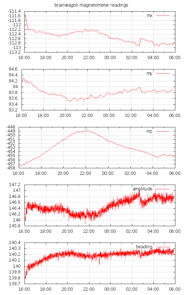
I’m really only just now trying to understand what the data actually means, and how the sensor is affected by things like temperature. This sensor is currently in my upstairs bathroom, which probably has a fairly wide temperature swing, is not level, and is probably closer to nearby metallic options than optimal. I’ll be letting this go in its current state to see if I can spot the diurnal (daily) variation in the heading. I suspect that most of the change in amplitude is actually due to changes in temperature. When I get a chance later this weekend, I’ll reset the device, and add a temperature sensor (probably a DS18B20) and record that along with the magnetic data, and maybe do some work to calibrate the sensor better.
I really like John’s site, and he also co-hosts a nifty geology podcast called the Don’t Panic Geocast. Definitely worth listening to, and inspiring me to learn more about geology, a subject that I admit I know relatively little about. Good stuff!
Capsule Review: The Adafruit Ultimate GPS Module
I picked up an Adafruit GPS module while at the Maker Faire. It’s a cool little module. I had a couple of old GPS modules: a Parallax PMB 648 and a Garmin 89, but this one is pretty nifty:
- It is small.
- It is breadboard friendly.
- It has a one pulse per second (1PPS) output for timing applications.
- It can output position/velocity information at up to 10Hz.
- It has a u.FL connector external antennas.
- It can be powered down by pulling an ENABLE pin low.
Lots of good features. I hooked it up tonight. My previous modules had a difficult time getting a lock inside, but this module had no difficulty at all. From a cold start, it had no problem locking. I hooked up the 1PPS output to my oscilloscope. It generates a nice 100ms positive pulse. The specifications say the timing jitter would be around 10ns. Very nice! That should be able to make a nice timebase to test the accuracy of the DS1307 module I was playing with yesterday. Data to come soon.
Rheoscopic Fluid (mica in suspension)
I mentioned in my Maker Faire wrap up post that I had spoken with Ben Krasnow, the science guru behind the Applied Science Youtube channel. If you haven’t watched his videos, by all means, go over there and give it a whirl. Between playing with chemicals, low temperatures, rockets, X rays, and electron microscope, it’s simply humbling.
He’s also a skilled woodworker, and build this rheoscopic coffee table. What is a rheoscope, you ask? A rheoscope is a device for measuring or detecting currents, usually in fluids. His table includes a spinning disk filled with a fluid that makes it easy to see the turbulence that goes on. If you go to as many science museums as I do, you’ll recognize the gadget. If you’ve tried to build furniture, you’ll recognize the craftsmenship.
This year, Ben brought some simpler fluid cells that are easier for people to construct. I cornered him and asked him what people used for the fluid that was in the cell. He mentioned that all sorts of particulates and fluids were used, including mica. I got home, and did a little web searching, and found that you could get a small container of powdered mica via Amazon Prime for under $10, so on Sunday I ordered some, and it arrived during my lunch hour. I couldn’t resist. I dumped about 1/4 of a teaspoon into a Smart Water bottle (purchased from the cafeteria) and filmed a quick demonstration.
And then recorded a longer explanatory video (only two minutes):
I suspect that the addition of some blue food coloring would enhance the contrast of the flow significantly.
Anyway, a kind of fun science fair project for a ten year old, or an aging computer scientist.
StarStack… Astrophotography with Cell Phones?
 Tom pointed me at this awesome article about an experiment run as part of the BBC programming Stargazing Live. Basically, they asked their viewers to go outside with their cell phones and take a picture of the night sky with their cell phones and upload the (almost entirely black) images to a website. They then used a process called “stacking” that basically aligned all the pixels and added them together. The net result was perhaps better than anyone has anyone had any expectation of getting. Very, very cool.
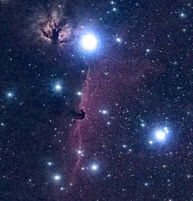
If you want to see the full image they constructed, click on the version below and you’ll get the resolution they achieved, including some views of the Great Nebula in Orion:

And, as it happens, the kind of thing that I could easily do with the hardware and software that I have lying around. I’m putting this onn my list of experiments to run, maybe with my iPhone, but more likely with the Pi Camera (easier to automate).
Addendum: Glancing at my copy of the Uranometria 2000, my “goto” star atlas, it’s clear that the picture I linked above has all the stars in the Uranometria, which is supposed to go down to about magnitude 9.75. Under dark skies, you’d only see down to magnitude 6 or so. Stars which are magnitude 9.75 are about 32 times dimmer, ordinarily you’d need to use a telescope with a 50mm aperature (a large-ish finder scope) to see these stars.
My first try at an inexpensive 0.96″ OLED display…
As my recent video showed, I have a lot of development boards. I also have a fair number of little boards that are useful to plugin to these development boards to accomplish various tasks. Yesterday, I received a little OLED board that I thought I’d try hooking up and let you know about my experience.
There are lots of boards out there that apparently use the same screen: a 0.96″ OLED display with a resolution of 128×64. I ordered this one from Amazon for only $9 with free shipping. The description is a little bit misleading: you can find versions of these kinds of boards that have 7 or 8 pins and use the SPI bus. This one has (and requires) only four pins, and uses the I2C bus. I’m no expert on the technical differences, but my general impression is that SPI is full duplex and can run at higher speed and at longer range, but requires individual chip select lines for each device, where the I2C bus uses chip addressing, so no additional wires need to be hooked up to select the proper target device. (If any of my genius readers care to correct me on that, feel free to leave a comment).
Here’s a picture of the module I got, as I tweeted it yesterday:
New OLED display…. pic.twitter.com/8B27BIOFXl
— Mark VandeWettering (@brainwagon) March 16, 2015
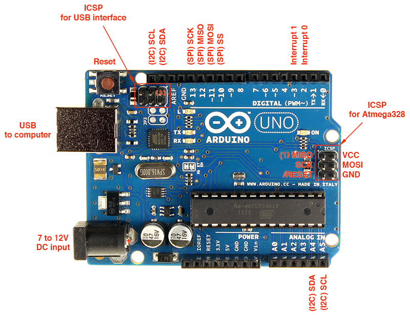
It’s safe to run on either 5v or 3.3v, without any level converters or other nonsense. I hooked it up to one of my Sparkfun RedBoard Arduino clones. I plugged it into a bread board, and then wired up the four connections. VCC goes to the 5V pin on the Redboard, GND goes to one of the Arduino grounds. The remaining two lines need to be hooked up to the SCL (serial clock) and SDA (serial data) lines on the Arduino. This caused me a minor bit of confusion: on an Arduino R3, those two pins are on A4 and A5.
On the RedBoard, these pins are split out separately onto separate pins near the AREF pin.
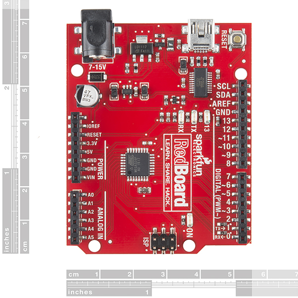
I connected them to the SCL/SDA connectors on the RedBoard. I suspect that on the Uno R3, A4/A5 are the connectors you’ll need. Other variants of the Arduino might need different pins.
And, of course you’ll need some software. It’s tempting to go to Adafruit for all things Arduino, but in this case it can be a bit of a mistake I think, or at least it might require a bit of tinkering. Adafruit sells their own OLED boards, but they are a bit more costly and are wired a bit differently, and I thought that might make their software a little trickier to configure.
Instead, I found the U8G graphics library. It’s fairly nice because it supports a wide variety of boards, and is self contained. If you download the Arduino code and unzip it into the Arduino library directory and restart the Arduino environment, you’ll see some examples installed. But if you load one and try to compile it, you’ll encounter an error: the examples aren’t configured for the particular board you need. To do that, you need to uncomment the right definition for the graphics device.
For this specific device, you want to delete the two slashes at the start of this line. This selects the I2C bus, and tells it to use the SSD1306 chip that is on the board. This one worked for me.
//U8GLIB_SSD1306_128X32 u8g(U8G_I2C_OPT_NONE); // I2C / TWI
So, I downloaded the “Graphics Test” example, made that modification, compiled it and downloaded it to the RedBoard. Voila
A pretty neat little display. I must say that it’s a bit too tiny for my old-guy eyes to read when the print is small (damn you presbyopia!) but It’s very sharp and clear. If you have need of such a device, this one seems inexpensive and easy to use. Check it out.
3/14/15
Happy Albert Einstein’s birthday! And we are just a few minutes away (in our time zone anyway) from 9:26. Huzzah!
I’m going to celebrate by making Shepard’s Pi(e) for dinner.
Increasing pyephem’s accuracy for satellite rise/set calculations…
A few years ago, I created my own Python implementation of the Plan13 satellite prediction code written by James Miller (G3RUH). The Plan13 algorithm isn’t very complicated: you can easily run it on processors like the Arduino (in fact, I used it for my ANGST satellite tracker) But somehow, I managed to misplace the source code for the Python version, probably on a hard drive for a computer that died, and so when I wanted to do some ISS calculations, I decided that I’d go ahead and use PyEphem, a much more complete package that can do all sorts of astronomical calculations, and which includes an implementation of the fairly standard SGP4 model.
It’s fairly simple to write some code to predict ISS passes from any position on earth. Here’s a quick example, with the TLEs for the ISS hard coded, as well as an observer position:
[sourcecode lang=”python”]
#!/usr/bin/env python
from math import degrees
import ephem
# create an observer
obs = ephem.Observer()
obs.lat = ‘38.0’
obs.lon = ‘-122’
obs.elevation = 100.
# create the iss object…
iss = ephem.readtle("ISS (ZARYA) ",
"1 25544U 98067A 15067.48441091 .00017347 00000-0 26069-3 0 9998",
"2 25544 51.6448 227.0292 0008846 83.1031 17.2346 15.54929647932364")
# figure out the next pass…
# only interested in rt (rise time), tt (transit time) and st (set time)
#
rt, razi, tt, televation, st, sazi = obs.next_pass(iss)
print "Rise Time: ", rt
print "Transit Time:", tt
print "Set Time: ", st
[/sourcecode]
But I was somewhat chagrined that if I ran this little snippet multiple times, I got different answers. Not by a lot, but by several seconds:
pi@blueberrypi ~ $ !.
./iss
Rise Time:    2015/3/8 22:30:12
Transit Time: 2015/3/8 21:00:52
Set Time:     2015/3/8 21:04:09
pi@blueberrypi ~ $ !!
./iss
Rise Time:    2015/3/8 22:30:12
Transit Time: 2015/3/8 21:00:53
Set Time:     2015/3/8 21:04:10
pi@blueberrypi ~ $ !!
./iss
Rise Time:    2015/3/8 22:30:13
Transit Time: 2015/3/8 21:00:53
Set Time:     2015/3/8 21:04:10
pi@blueberrypi ~ $ !!
./iss
Rise Time:    2015/3/8 22:30:03
Transit Time: 2015/3/8 21:00:49
Set Time:     2015/3/8 21:04:11
Digging in the code, it’s not hard to see what’s going on. The code is stepping forward by intervals of about 1 minute, trying to catch the satellite as it peaks over the horizon. When it does, it then uses twenty iterations of the secant method to find the point where the satellite crosses zero altitude. But there is an early out: if the interval drops below ten seconds, it goes ahead and exists. Similarly, it only locates the time of the transit to within 15 seconds. But these can be fixed with some quick, and probably undisciplined changes to the code will make things behave better.
Both edits are in the file riset_cir.c which is part of libastro-3.7.5 (your version might change, but will probably be the same). Near the top you’ll find the declaration for TMACC
[sourcecode lang=”C”]
#define TMACC (10./3600./24.0) /* convergence accuracy, days */
[/sourcecode]
Change this to 0.5 seconds instead.
[sourcecode lang=”C”]
#define TMACC (0.5/3600./24.0) /* convergence accuracy, days */
[/sourcecode]
You might want to increase MAXPASSES in the find_0alt function, but I had no difficulty with leaving it at 20.
Similarly, we need to change the error in find_transit:
[sourcecode lang=”C”]
static int
find_transit (double dt, Now *np, Obj *op)
{
#define MAXLOOPS 10
#define MAXERR (0.25/60.) /* hours */
[/sourcecode]
The number of iterations is pretty low (just 10) and the MAXERR was 15 seconds. I decided to add some iterations to ensure convergence, and to set the MAXERR to be just one second.
[sourcecode lang=”C”]
static int
find_transit (double dt, Now *np, Obj *op)
{
#define MAXLOOPS 20
#define MAXERR (1./3600.) /* hours */
[/sourcecode]
With these changes in place, you get times which are accurate to around one second. Note: I do not mean to imply that these numbers are somehow absolutely better. It is known that the SGP4 model can only locate satellites to errors of around 1km per day at best, so trying to converge them to insane levels of accuracy isn’t meaningful. But for my application, I want to count down to transits, and having the estimate jump around by a few seconds made the count down look funny. Of course, I could have just computed the times once, and used that, but I still think it’s kind of odd that the estimates vary by a human discernable amount depending solely on what time you decide to try to compute from. This additional accuracy makes the program a very tiny bit slower, but is worth it for my application.
Addendum: A few more lines of code make the code a bit more useful. This now outputs the next pass expressed in the localtime rather than UTC, and gives you a bit of a countdown.
[sourcecode lang=”python”]
#!/usr/bin/env python
from math import degrees
import ephem
import datetime
# create an observer
obs = ephem.Observer()
obs.lat = ‘38.0’
obs.lon = ‘-122’
obs.elevation = 100.
# create the iss object…
iss = ephem.readtle("ISS (ZARYA) ",
"1 25544U 98067A 15067.48441091 .00017347 00000-0 26069-3 0 9998",
"2 25544 51.6448 227.0292 0008846 83.1031 17.2346 15.54929647932364")
# figure out the next pass…
# only interested in rt (rise time), tt (transit time) and st (set time)
#
n = ephem.now()
rt, razi, tt, televation, st, sazi = obs.next_pass(iss)
print "%d" % round((rt – n) * 3600 * 24), "seconds until the next pass."
rt = ephem.localtime(rt).strftime("%x %X")
tt = ephem.localtime(tt).strftime("%x %X")
st = ephem.localtime(st).strftime("%x %X")
print "Rise Time: ", rt, "Azimuth: %5.1f" % degrees(razi)
print "Transit Time:", tt, "Elevation: %5.1f" % degrees(televation)
print "Set Time: ", st, "Azimuth: %5.1f" % degrees(sazi)
[/sourcecode]
Addendum2: A few more lines of code fetches a current set of orbital elements from celestrak.com. A future revision of this will probably cache a local copy of these orbital elements so you don’t unnecessarily hammer their server.
[sourcecode lang=”python”]
#!/usr/bin/env python
from math import degrees
import ephem
import datetime
import urllib2
req = urllib2.Request("http://celestrak.com/NORAD/elements/amateur.txt")
response = urllib2.urlopen(req)
data = response.read().splitlines()
objs = []
for idx in range(0, len(data), 3):
objs.append(ephem.readtle(data[idx], data[idx+1], data[idx+2]))
# create an observer
obs = ephem.Observer()
obs.lat = ‘38.0’
obs.lon = ‘-122’
obs.elevation = 100.
# create the iss object…
iss = ephem.readtle("ISS (ZARYA) ",
"1 25544U 98067A 15067.48441091 .00017347 00000-0 26069-3 0 9998",
"2 25544 51.6448 227.0292 0008846 83.1031 17.2346 15.54929647932364")
# figure out the next pass…
# only interested in rt (rise time), tt (transit time) and st (set time)
#
tlist = []
for obj in objs:
r = obs.next_pass(obj)
tlist.append((r[0], obj, r))
tlist.sort()
for t, obj, r in tlist:
n = ephem.now()
rt, razi, tt, televation, st, sazi = r
print obj.name
print "%d" % round((rt-n) * 3600 * 24), "seconds until the next pass."
rt = ephem.localtime(rt).strftime("%x %X")
tt = ephem.localtime(tt).strftime("%x %X")
st = ephem.localtime(st).strftime("%x %X")
print "Rise Time: ", rt, "Azimuth: %5.1f" % degrees(razi)
print "Transit Time:", tt, "Elevation: %5.1f" % degrees(televation)
print "Set Time: ", st, "Azimuth: %5.1f" % degrees(sazi)
print
[/sourcecode]
The output is now a list of all the amateur satellites that it fetched, sorted in order of the passes which are soonest appear first.
BEESAT-2
410 seconds until the next pass.
Rise Time:    03/08/15 18:33:03 Azimuth:   272.2
Transit Time: 03/08/15 18:37:54 Elevation:   8.1
Set Time:     03/08/15 18:42:45 Azimuth:     9.4

CUBESAT XI-V (CO-58)
526 seconds until the next pass.
Rise Time:    03/08/15 18:34:59 Azimuth:    31.0
Transit Time: 03/08/15 18:41:08 Elevation:  16.4
Set Time:     03/08/15 18:47:16 Azimuth:   153.1

XIWANG-1 (HOPE-1)
1228 seconds until the next pass.
Rise Time:    03/08/15 18:46:41 Azimuth:    91.6
Transit Time: 03/08/15 18:53:13 Elevation:   8.5
Set Time:     03/08/15 18:59:45 Azimuth:     6.5

OSCAR 7 (AO-7)
1251 seconds until the next pass.
Rise Time:    03/08/15 18:47:04 Azimuth:   229.2
Transit Time: 03/08/15 18:54:42 Elevation:   8.5
Set Time:     03/08/15 19:02:20 Azimuth:   317.9

AAUSAT3
2080 seconds until the next pass.
Rise Time:    03/08/15 19:00:54 Azimuth:    29.7
Transit Time: 03/08/15 19:07:39 Elevation:  19.3
Set Time:     03/08/15 19:14:25 Azimuth:   157.0

PCSAT (NO-44)
2515 seconds until the next pass.
Rise Time:    03/08/15 19:08:08 Azimuth:   173.2
Transit Time: 03/08/15 19:15:24 Elevation:  24.3
Set Time:     03/08/15 19:22:39 Azimuth:    41.1

CUTE-1.7+APD II (CO-65)
2940 seconds until the next pass.
Rise Time:    03/08/15 19:15:14 Azimuth:    81.8
Transit Time: 03/08/15 19:17:56 Elevation:   1.9
Set Time:     03/08/15 19:20:37 Azimuth:    31.8

JAS-2 (FO-29)
2956 seconds until the next pass.
Rise Time:    03/08/15 19:15:30 Azimuth:   255.5
Transit Time: 03/08/15 19:19:08 Elevation:   2.2
Set Time:     03/08/15 19:22:47 Azimuth:   307.5

M-CUBED & EXP-1 PRIME
3635 seconds until the next pass.
Rise Time:    03/08/15 19:26:49 Azimuth:   354.1
Transit Time: 03/08/15 19:32:20 Elevation:  12.4
Set Time:     03/08/15 19:37:52 Azimuth:   247.0

MOZHAYETS 4 (RS-22)
3940 seconds until the next pass.
Rise Time:    03/08/15 19:31:54 Azimuth:   347.2
Transit Time: 03/08/15 19:37:10 Elevation:   9.9
Set Time:     03/08/15 19:42:26 Azimuth:   248.6

CUBESAT XI-IV (CO-57)
4134 seconds until the next pass.
Rise Time:    03/08/15 19:35:08 Azimuth:   194.6
Transit Time: 03/08/15 19:42:31 Elevation:  27.0
Set Time:     03/08/15 19:49:53 Azimuth:   334.6

HAMSAT (VO-52)
4222 seconds until the next pass.
Rise Time:    03/08/15 19:36:36 Azimuth:   235.6
Transit Time: 03/08/15 19:40:29 Elevation:   4.5
Set Time:     03/08/15 19:44:22 Azimuth:   310.9

PRISM (HITOMI)
4468 seconds until the next pass.
Rise Time:    03/08/15 19:40:41 Azimuth:    13.2
Transit Time: 03/08/15 19:47:14 Elevation:  82.2
Set Time:     03/08/15 19:53:46 Azimuth:   192.3

CUTE-1 (CO-55)
4562 seconds until the next pass.
Rise Time:    03/08/15 19:42:16 Azimuth:   198.2
Transit Time: 03/08/15 19:49:30 Elevation:  23.6
Set Time:     03/08/15 19:56:44 Azimuth:   332.9

STRAND-1
4714 seconds until the next pass.
Rise Time:    03/08/15 19:44:47 Azimuth:    18.5
Transit Time: 03/08/15 19:52:18 Elevation:  49.9
Set Time:     03/08/15 19:59:48 Azimuth:   181.1

BEESAT-3
4722 seconds until the next pass.
Rise Time:    03/08/15 19:44:55 Azimuth:   342.9
Transit Time: 03/08/15 19:44:56 Elevation:  -0.0
Set Time:     03/08/15 19:44:56 Azimuth:   342.9

YUBILEINY (RS-30)
5115 seconds until the next pass.
Rise Time:    03/08/15 19:51:28 Azimuth:   279.5
Transit Time: 03/08/15 19:57:25 Elevation:   3.7
Set Time:     03/08/15 20:03:21 Azimuth:   342.8

TRITON-1
5411 seconds until the next pass.
Rise Time:    03/08/15 19:56:24 Azimuth:    92.7
Transit Time: 03/08/15 20:00:09 Elevation:   3.9
Set Time:     03/08/15 20:03:54 Azimuth:    25.1

UOSAT 2 (UO-11)
6509 seconds until the next pass.
Rise Time:    03/08/15 20:14:43 Azimuth:    95.0
Transit Time: 03/08/15 20:18:33 Elevation:   4.5
Set Time:     03/08/15 20:22:23 Azimuth:    22.8

SEEDS II (CO-66)
6557 seconds until the next pass.
Rise Time:    03/08/15 20:15:30 Azimuth:   127.3
Transit Time: 03/08/15 20:21:07 Elevation:  16.4
Set Time:     03/08/15 20:26:43 Azimuth:     6.7

UWE-3
6694 seconds until the next pass.
Rise Time:    03/08/15 20:17:48 Azimuth:    76.8
Transit Time: 03/08/15 20:20:03 Elevation:   1.3
Set Time:     03/08/15 20:22:18 Azimuth:    35.9

RADIO ROSTO (RS-15)
7326 seconds until the next pass.
Rise Time:    03/08/15 20:28:20 Azimuth:   128.2
Transit Time: 03/08/15 20:36:14 Elevation:   6.0
Set Time:     03/08/15 20:44:09 Azimuth:    56.8

GOMX 1
7721 seconds until the next pass.
Rise Time:    03/08/15 20:34:55 Azimuth:   139.6
Transit Time: 03/08/15 20:41:44 Elevation:  28.3
Set Time:     03/08/15 20:48:33 Azimuth:     0.7

CUBEBUG-2 (LO-74)
9556 seconds until the next pass.
Rise Time:    03/08/15 21:05:29 Azimuth:   126.2
Transit Time: 03/08/15 21:11:12 Elevation:  15.9
Set Time:     03/08/15 21:16:56 Azimuth:     7.5

VELOX-PII
9914 seconds until the next pass.
Rise Time:    03/08/15 21:11:28 Azimuth:   125.2
Transit Time: 03/08/15 21:17:05 Elevation:  15.3
Set Time:     03/08/15 21:22:43 Azimuth:     8.0

FUNCUBE-1 (AO-73)
9936 seconds until the next pass.
Rise Time:    03/08/15 21:11:49 Azimuth:   118.8
Transit Time: 03/08/15 21:17:04 Elevation:  11.9
Set Time:     03/08/15 21:22:20 Azimuth:    11.1

ZACUBE-1 (TSHEPISOSAT)
10153 seconds until the next pass.
Rise Time:    03/08/15 21:15:26 Azimuth:   121.9
Transit Time: 03/08/15 21:20:52 Elevation:  13.4
Set Time:     03/08/15 21:26:17 Azimuth:     9.6

DELFI-C3 (DO-64)
11107 seconds until the next pass.
Rise Time:    03/08/15 21:31:21 Azimuth:   142.9
Transit Time: 03/08/15 21:37:20 Elevation:  29.2
Set Time:     03/08/15 21:43:19 Azimuth:   359.6

HUMSAT-D
12799 seconds until the next pass.
Rise Time:    03/08/15 21:59:32 Azimuth:   133.5
Transit Time: 03/08/15 22:05:21 Elevation:  20.4
Set Time:     03/08/15 22:11:09 Azimuth:     4.0

EAGLE 2
13942 seconds until the next pass.
Rise Time:    03/08/15 22:18:36 Azimuth:   136.2
Transit Time: 03/08/15 22:24:17 Elevation:  22.0
Set Time:     03/08/15 22:29:58 Azimuth:     3.0

CUBEBUG-1 (CAPITAN BETO)
15152 seconds until the next pass.
Rise Time:    03/08/15 22:38:45 Azimuth:   129.1
Transit Time: 03/08/15 22:44:45 Elevation:  18.7
Set Time:     03/08/15 22:50:44 Azimuth:     4.6

SPROUT
15611 seconds until the next pass.
Rise Time:    03/08/15 22:46:24 Azimuth:    92.6
Transit Time: 03/08/15 22:50:05 Elevation:   4.0
Set Time:     03/08/15 22:53:46 Azimuth:    24.0

JUGNU
16144 seconds until the next pass.
Rise Time:    03/08/15 22:55:18 Azimuth:   204.1
Transit Time: 03/08/15 23:00:40 Elevation:   6.1
Set Time:     03/08/15 23:06:02 Azimuth:   124.2

DUCHIFAT-1
16575 seconds until the next pass.
Rise Time:    03/08/15 23:02:29 Azimuth:    35.0
Transit Time: 03/08/15 23:07:53 Elevation:  12.7
Set Time:     03/08/15 23:13:17 Azimuth:   148.7

SRMSAT
17209 seconds until the next pass.
Rise Time:    03/08/15 23:13:03 Azimuth:   176.4
Transit Time: 03/08/15 23:15:40 Elevation:   1.1
Set Time:     03/08/15 23:18:17 Azimuth:   139.8

SWISSCUBE
18892 seconds until the next pass.
Rise Time:    03/08/15 23:41:05 Azimuth:    73.7
Transit Time: 03/08/15 23:43:37 Elevation:   1.4
Set Time:     03/08/15 23:46:09 Azimuth:    31.4

SAUDISAT 1C (SO-50)
19177 seconds until the next pass.
Rise Time:    03/08/15 23:45:51 Azimuth:   170.5
Transit Time: 03/08/15 23:52:00 Elevation:  17.7
Set Time:     03/08/15 23:58:10 Azimuth:    47.9

BEESAT
19303 seconds until the next pass.
Rise Time:    03/08/15 23:47:57 Azimuth:    77.8
Transit Time: 03/08/15 23:50:51 Elevation:   2.0
Set Time:     03/08/15 23:53:45 Azimuth:    28.8

TISAT 1
19890 seconds until the next pass.
Rise Time:    03/08/15 23:57:44 Azimuth:   141.2
Transit Time: 03/09/15 00:03:57 Elevation:  28.7
Set Time:     03/09/15 00:10:10 Azimuth:   359.5

ITUPSAT 1
21056 seconds until the next pass.
Rise Time:    03/09/15 00:17:09 Azimuth:   104.3
Transit Time: 03/09/15 00:22:11 Elevation:   8.1
Set Time:     03/09/15 00:27:12 Azimuth:    14.2

KKS-1 (KISEKI)
24703 seconds until the next pass.
Rise Time:    03/09/15 01:17:56 Azimuth:    96.4
Transit Time: 03/09/15 01:22:04 Elevation:   5.2
Set Time:     03/09/15 01:26:12 Azimuth:    20.4

LUSAT (LO-19)
25871 seconds until the next pass.
Rise Time:    03/09/15 01:37:24 Azimuth:    29.2
Transit Time: 03/09/15 01:44:13 Elevation:  20.0
Set Time:     03/09/15 01:51:01 Azimuth:   157.9

ITAMSAT (IO-26)
26776 seconds until the next pass.
Rise Time:    03/09/15 01:52:30 Azimuth:    42.8
Transit Time: 03/09/15 01:57:50 Elevation:   7.6
Set Time:     03/09/15 02:03:10 Azimuth:   133.0

TECHSAT 1B (GO-32)
27579 seconds until the next pass.
Rise Time:    03/09/15 02:05:52 Azimuth:    41.3
Transit Time: 03/09/15 02:11:26 Elevation:   8.3
Set Time:     03/09/15 02:17:00 Azimuth:   134.4

HORYU 2
31680 seconds until the next pass.
Rise Time:    03/09/15 03:14:13 Azimuth:    41.7
Transit Time: 03/09/15 03:19:13 Elevation:   8.3
Set Time:     03/09/15 03:24:13 Azimuth:   137.6

ISS (ZARYA)
38130 seconds until the next pass.
Rise Time:    03/09/15 05:01:43 Azimuth:   115.2
Transit Time: 03/09/15 04:15:25 Elevation: -74.9
Set Time:     03/09/15 05:01:43 Azimuth:   115.2
Addendum3: Hmm. If you look carefully, the last entry in the test output is bogus: the time of maximum elevation does not fall between the rise and set time, and the elevation is negative. Staring at the code some more, I’m now worried about the logic of the root finder. I’ll have to ponder it some more.
A pair of geeky Advent calendars…
Advent is the season observed in many Christian traditions that is a time of expectant waiting and preparation for Christmas. When I was young, we’d have an Advent calendar, which counted down the days to Christmas, and would gift us with a little chocolate or candy each day.
While I am no longer religious, the idea is kind of cool: to take a little time out of each day and enjoy a tasty treat of some sort, and think of the upcoming holiday. A couple of cool examples have crossed my desk…
I like to experiment with embedded controllers, machine emulation and operating systems, so I am of course familiar with QEMU, but in case you are not: QEMU is a generic and open source machine emulator and virtualizer. It allows you simulate machines and run code written for one machine (say, an ARM board) on your PC using virtual hardware peripherals. It also serve as a “virtualizer”, which basically means that if you have an x86 Linux box, you can run a different x86 operating system on the same hardware, at very nearly native performance. In short, it’s pretty awesome.
If you like this kind of thing, you should check o ut The QEMU Advent Calendar 2014. It presents a new QEMU disk image each day until Christmas, enabling you to play with new operating systems, programming languages and graphical goodies. For instance, Day 6 is a tiny image that generates Julia sets.

Other days allow you to boot ancient versions of Slackware Linux, run an Atari ST emulator inside QEMU, and even play Zork. Awesome.
But even greater than that is the offering by Alan, VK2ZA7. Back in 2011, he did a series of 24 Youtube videos that each described a small electronic circuit that he tinkered together during the Christmas season. Many of them had to do with generating small bits of test equipment or illustrate some cool little circuits. Ones that I liked were his LED based transmitter/receiver:
and this nice little crystal radio, very traditional, with a cobweb style coil wound with Litz wire, but with a polyvaricon variable capacitor instead of the traditional 365pf variable cap.
What’s awesome is that after a hiatus of a couple years, Alan is back in 2014 with new projects. Very, very cool.
I particularly liked this one on building variable capacitors (a laser cutter would be helpful). I hadn’t seen this kind of geometry in one before, and Alan’s patter is very interesting.
A particularly useful little bit of tech for us radio tinkerers:
I’ll be checking back each day until Christmas. Thanks Alan!
Photos from the eclipse…
Okay, these are the best of the photos that I snapped during yesterdays annular solar eclipse (well, it was really only a partial eclipse here). We had just left the Maker Faire, and were in the parking lot of Oracle on 10 Twin Dolphin Drive in Redwood City, CA. I took out my 4″ Meade Maksutov telescope, along with a full aperature solar filter and a 25mm eyepiece. To take the pictures, I used a Fuji W1 camera, held up to the eyepiece, set in manual mode with an exposure of 1/100th of a second and f/4. Alignment was tricky and twitchy, and there are more crappy photos than good ones. These aren’t particularly good, or sharp, but heck, they are mine, and as a reminder of a kind of neat event, they work just fine.


Upcoming Total Lunar Eclipse
Yep, there is an upcoming total lunar eclipse this Saturday, on the morning of Dec 10. It will be the last total lunar eclipse visible from San Francisco until April of 2014, so I think I’ll be trying to get up and see if I can view it and take some snapshots. From San Francisco, will enter the penumbra at 3:34 local time. You should start seeing it enter partial eclipse around 4:46, and it will begin totality around 6:06 (at only 12 degrees of altitude). Totality ends around 6:57, with the moon at about 3 degrees altitude.
I’ll probably get out my aircraft spotting binocs, and try some ghetto “through the eyepiece” photography. Stay tuned.
Some simple circuits with solar cells…
My tinkering with my ATtiny13 based pumpkin circuit had me thinking that perhaps I should try to make something similar, but solar powered. Luckily, Windell had already anticipated my needs, and had put up a nice simple page with some circuits to experiment with. If you want a simple solar battery charger, or a simple solar powered microcontroller, try checking this out:
Nyle Steiner finds and demonstrates a memristor
Nyle Steiner, of the Spark Bang Buzz blog has been at it again, demonstrating cool electrical/electronic devices that are homebrewed. This time he constructed his own memristor.
If you aren’t up on electronics, you might not have heard of memristors before. While Leon Chua proposed that such a circuit element was possible, they weren’t actually created in a lab until 2008. But what is a memristor? It’s a circuit element whose resistance depends on the sum of the charge flowing through it. In other words, if you pass a voltage through a memristor in one direction, it’s resistance increases. If you pass a voltage through the other way, it decreases. But if you stop the voltage entirely, the memristor “remembers” the previous value it had, and will keep the same resistance it had when the charge was cut.
Amazingly, Nyle Steiner observed this memory effect in some brass shell casings which had been oxidized in a sulfur environment (I’m no chemist, so I won’t try to explain that part) over 10 years ago. He made this short video demonstrating such a memristor using both a curve tracer (which may take a few minutes of though to understand exactly what is going on) but also through a very basic circuit demonstrating how the memristor can “remember” a single bit and turn an LED on and off. If you didn’t know that memristor’s existed, you’d probably be forced to try to explain the behavior of the circuit in terms of capacitance: but unlike capacitance, the memristor doesn’t need to be refreshed to maintain its state. You’d find it rather puzzling, to be sure.
Awesome stuff.
Electromagnetic Propulsion of Ships and Submarines
The other day, I was watching The Hunt For Red October on TV. Through some odd coincidence, today I found a link to an article that was published in Popular Science back in 1966 on a silent electromagnetic drive for submarines, just like the “caterpillar drive” of the Red October. I didn’t realize that this was a real thing! It seems like it would be a fun experiment to build an demonstration showing this effect, and indeed, this page links to some articles that would seem to be helpful.
Electromagnetic Propulsion Ships, Submarines: patents & articles
Bookmarked for later perusal.